
OPTIMAL SPANNING TREES MIXTURE BASED PROBABILITY
APPROXIMATION FOR SKIN DETECTION
Sanaa El Fkihi
1,2
, Mohamed Daoudi
1
1
GET/TELECOM Lille1, LIFL (UMR USTL-CNRS 8022), Cit´e Scientifique - Rue Guglielmo Marconi , Villeneuve d’Ascq, France
Driss Aboutajdine
2
2
GSCM
LRIT Faculty of Sciences, University Mohammed V, Rabat, Morocco
Keywords:
Optimal spanning tree, dependency tree, mixture of trees, skin detection, classification, probability graphical
models, tree distributions.
Abstract:
In this paper we develop a new skin detection algorithm for learning in color images. Our contribution is based
on the Optimal Spanning Tree distributions that are widely used in many optimization areas. Thus, by making
some assumptions we propose the mixture of the Optimal Spanning Trees to approximate the true Skin (or
Non-Skin) class probability in a supervised algorithm.
The theoretical proof of the Optimal Spanning Trees’ mixture is drawn. Furthermore, the performance of our
method is assessed on the Compaq database by measuring the Receiver Operating Characteristic curve and its
under area. These measures have proved better results of the proposed model compared with the results of a
random Optimal Spanning Tree model and the baseline one.
1 INTRODUCTION
Tree distributions are well-known machine learning
solutions to deal with probability estimation problem.
(Chow and Liu, 1968) supplied an heuristic to find
maximum likelihood Markov Trees called Optimal
Dependency Trees or Optimal Spanning Trees. The
heuristic problem aimed to provide an efficient al-
gorithm to find a maximum-weight spanning tree
(MWST) proved to be the optimal one in the sense
of Maximum Likelihood criterion. Since then, many
methods based on that work have been extended: the
polytrees (Pearl, 1988); the mixtures of trees with ob-
served structure variable (Geiger, 1992); the mixture
of Tree-Union (Torsello and Hancock, 2006).
In addition, the authors of (Meila and Jordan, 2000)
proposeda mixture of trees with hidden structurevari-
able. When the variable is a class label, the mixture
model is the bayesian network. Otherwise, the class
variable is considered as the training data in an unsu-
pervised algorithm used to learn the mixed trees.
The MWST has applications in many optimiza-
tion areas. However, this tree is not usually unique.
Indeed, considering a graph with identically weighted
edges, all spanning trees are MWSTs. Consequently,
different tree probability distributions can approxi-
mate on the best way the true probability distribution.
In many domains what is required is not necessarily
the best spanning tree, but rather a ’perfect’ one with
some other properties that may be difficult to quan-
tify. So, what could be the ’perfect’ spanning tree in
the skin detection application?
Research has been performed on the detection of
human skin pixels in color images by the use of var-
ious statistical color models (Jedynak et al., 2005),
such Gaussian mixture and histograms (Jones and
Rehg, 1999). The comparison results of these lat-
ters, estimated with EM algorithm, found that the
histogram model is slightly superior in terms of skin
classification for the standard 24-bit RGB color space.
Moreover, in addition to the semi-supervised ap-
proach for learning the structure of Bayesian network
classifiers based on an Optimal Spanning Tree (Sebe
et al., 2004), the Best-Tree distribution algorithm ap-
proximating the skin and non skin probability distrib-
utions has been also proposed (ElFkihi et al., 2006).
Since quantifying other ’perfect’ Skin (or Non-
Skin) tree properties is unobvious, our aim is to pro-
vide a learning algorithm for skin/non-skin classi-
fication, seeking a spanning tree which emphasizes
382
El Fkihi S., Daoudi M. and Aboutajdine D. (2007).
OPTIMAL SPANNING TREES MIXTURE BASED PROBABILITY APPROXIMATION FOR SKIN DETECTION.
In Proceedings of the Second International Conference on Computer Vision Theory and Applications - IFP/IA, pages 382-385
Copyright
c
SciTePress

the data dependencies’ degrees, and approximates the
probability distribution; without adding information.
The next section points out the mathematical for-
mulation of the studied problem. Section 3 details our
approach while section 4 is devoted to experiments
and results. Conclusions are postponed to section 5.
2 PROBLEM FORMULATION
In the RGB color space, we note x
s
the color of a
pixel s. y
s
= 1 is a skin pixel label and y
s
= 0 a
non-skin pixel label. Let r be an integer value, we
define the following neighborhood system:
V
r
s
= {(i, j)/|i− i
s
| < r,| j − j
s
| < r} \ {(i
s
, j
s
)} (1)
We consider (x
1
,x
2
,... ,x
h
2
) an observation vector
standing for an image patch (h × h,h = 2r − 1). This
vector is decomposed until a low-level elements; and
the resultant vector is x = (x
1
,. .. ,x
n
), where n = 3h
2
.
In practice, the joint probability distribution
P(x,y
s
) is unknown, instead we have a seg-
mented Database which is a collection of samples
{(x
(1)
,y
(1)
),... ,(x
(N)
,y
(N)
)} that we suppose inde-
pendent; x
( j)
is a color image, and y
( j)
is its binary
skinness image. Our objective is to construct proba-
bilistic classifiers that represent the posterior proba-
bilities P(y
s
= i|x) (i = 0, 1) at s, given its neighbors.
We consider the observation vector x and G(V,E)
its corresponding undirect graph representation. V is
the vertex set representing observations and E is the
edge set enclosing dependencies between the obser-
vations. In case G is a tree, noted T, the formulation
probability represented by such structure and approxi-
mating the true probability P is given in (Pearl, 1988):
P(x) ⋍
∏
(u∼v)∈T
P
uv
(x
u
,x
v
)
P
u
(x
u
)P
v
(x
v
)
∏
u∈V
P
u
(x
u
) (2)
where P
u
(x
u
) and P
uv
(x
u
,x
v
) are marginals of P(x),
and u ∼ v means two neighboring vertices u and v.
(Chow and Liu, 1968) calculated the Kullback-
Leibler (KL) divergence of the true probability and
the one approximated by a tree. They proved that
minimizing this distance is equal to maximizing:
W
T
=
∑
(u∼v)∈T
KL(P
uv
(x
u
,x
v
),P
u
(x
u
)P
v
(x
v
)) (3)
which is the weight of the spanning tree T. An arbi-
trary solution is readily obtained in polynomial time
by simple greedy algorithms (Bach and Jordan, 2003),
and it is called an Optimal Spanning Tree (OST).
The OSTs of a graph emphasize the important depen-
dencies between its different components. Hence, we
propose the next mixture of the tree probabilities:
∑
T∈Θ
λ(T)P(x|T) (4)
with Θ is the set of all OSTs, and P(x|T) is the prob-
ability of a tree T while λ(T) is a mixture coefficient
verifying
∑
T∈Θ
λ(T) = 1 and λ(T) ≥ 0.
Hence, the probability classifier we are looking for
is the mixture probability that we have to compute by
determining λ(T) and solving the likelihood function:
T
mix
= argmax
T
′
n
∑
i=1
∑
T∈Θ
log(λ(T)P(x
i
|T)) (5)
where a tree T
′
represents a mixture probability.
3 THE MIXTURE MODEL
First, we propose the next theorem:
Theorem
1 The true probability distribution (P(x))
is most efficiently approximated by the tree proba-
bility distribution (P(x|T
mix
)) obtained by the mix-
ture of Optimal Spanning Trees (T
mix
) than the one
(P(x|T
op
)) obtained by an Optimal Spanning Tree
(T
op
). Otherwise:
KL(P(x),P(x|T
mix
)) ≤ KL(P(x),P(x|T
op
)) (6)
We conclude that our proposal is justified because
of its improvementcompared with an OST model (our
theorem proof is postponed to the appendix).
In the next, we will discuss two main steps that are
the training and the inference.
3.1 Training Step
In order to select the OSTs we have to list all the graph
spanning trees, which is algorithmically difficult. To
deal with this, we suggest to select K OSTs (K ∈ N
∗
)
using the K-Best-Spanning-Trees algorithm given in
(Katoh et al., 1981) with respect to this constraint:
W
T
i
= argmax
T
W
T
, 1 ≤ i ≤ k (7)
where W
T
i
is the weight of the OST numbered i and
W
T
is the weight of the spanning tree T.
Let noted the set of the selected trees by Θ
k
, and
P(x|y
s
= 1) by p(x), and P(x|y
s
= 0) by q(x).
The procedure to obtain the Skin mixture of the
OSTs distribution (T
mix
) is:
Procedure
1 Distribution of the skin Optimal Span-
ning Trees’ mixture.
• Input : Dataset
n
x
(1)
,y
(1)
,··· ,
x
(n)
,y
(n)
o
.
1. Define the neighborhood system (equation(1)).
2. Construct the vector of observations x.
3. Build a complete non-oriented graph of x.
4. Let two different vertices u and v. Use the empiri-
cal estimators to compute p
u
(x
u
) and p
uv
(x
u
,x
v
).
5. Compute the edge cost between u and v:
KL(p
uv
(x
u
,x
v
), p
u
(x
v
)p
v
(x
v
)) (8)
6. Apply the K-Best-Spanning-Trees algorithm.
7. Estimate the mixture coefficients (section 3.2)
• Output
: T
mix
and the mixture coefficients.
3.2 Parameters’ Estimation
To estimate the mixture coefficients of Skin OSTs’
mixture, we propose a graphical model allowing to re-
store each tree of the optimal considered ones. First,
because of the fact that the different trees have the
same vertices, the vertex set of the graph is the same
as the one of these trees. Second, so as not to loose
any information brought by the different trees, we
suggest to keep all the edges of these ones. Further-
more, we propose this edge cost between u and v:
W
u∼v
= KL(pmix
uv
(x
u
,x
v
), pmix
u
(x
u
)pmix
v
(x
v
))
(9)
where pmix
u
and pmix
uv
are marginals of the Skin
mixture probability defined like in equation (4), pmix.
Then, we suggest to use the EM algorithm to find the
Skin OST performing the mixture model, such: the E
step estimates the λ(T) and the M step re-estimates
the parameters of the model to solve the equation (5).
3.3 Inference
The state of the pixel y
s
given the observation vector
x, is:
P(y
s
= i|x) ≈
∑
T∈Θ
k
λ(T)P(y
s
= i|x, T);i = 0, 1 (10)
By applying the Bayes’ rule on each T ∈ Θ
k
, we
obtain:
P(y
s
= 0|x) ≈
∑
T∈Θ
k
λ(T)q(y
s
= 0|T)q(x|T)
p(y
s
= 1|T)p(x|T) + q(y
s
= 0|T)q(x|T)
(11)
P(y
s
= 1|x) ≈
∑
T∈Θ
k
λ(T)p(y
s
= 1|T)p(x|T)
p(y
s
= 1|T)p(x|T) + q(y
s
= 0|T)q(x|T)
(12)
All the elements of equations (11) and (12) are previ-
ously computed in the procedure 1.
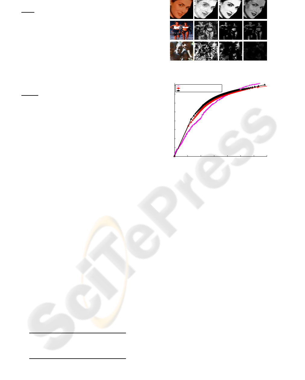
Figure 1: Some inputs (color images) and outputs (grayscal-
ing images) of the three compared models.
0 0.01 0.02 0.03 0.04 0.05 0.06 0.07
0
0.1
0.2
0.3
0.4
0.5
0.6
0.7
0.8
False positive rate
True positive rate
Baseline model
Chow & Liu Optimal−Spanning−Tree model
Mixture of Optimal−Spanning−Trees model
Figure 2: The ROC curves of the three compared models.
4 EXPERIMENTS AND RESULTS
All experiments are made on the Compaq Database
(Jones and Rehg, 1999) which is split into two almost
equal parts randomly (the training and the test parts).
We define the neighborhood system of a pixel in
which r = 2. In order to evaluate the performances of
the proposed model we compare it to two other mod-
els: the model based on a random OST (Chow and
Liu, 1968) and the baseline one in which pixels are
considered independent (Jones and Rehg, 1999).
In figure 1, the second column corresponds to the
outputs of the OST model. The outputs of our pro-
posed model are shown in the third column while the
ones of the baseline are given in the fourth column.
We present the Receiver Operating Characteris-
tic (ROC) curves of the considered models (figure 2);
where false positive rate is the proportion of non-skin
pixels classified as skin whereas detection rate is the
proportion of skin pixels classified as skin.
The ROC curves show an improvement of the perfor-
mance for all false positive rate of the mixture model
compared to an OST one. Especially, an increase skin
detection of the mixture model compared to the base-
line is detected from 0.04% to 0.48% false positive.
In addition, using [0;0.07], the area under the ROC
curve (AUC) is equals to 0.0296 for the Baseline,
0.0382 for the OST, and 0.0414 for our approach.

Figure 3 shows some cases where our detector
failed due to over-exposure, or to skin-like color.
Figure 3: Some examples where our mixture model fails.
5 CONCLUSION
In this paper, we have presented a new algorithm de-
voted to the mixture of OSTs to deal with the prob-
lems of either classification or probability approxima-
tion of skin/non-skin. It emphasizes and takes account
of the useful information of each existing OST.
A theoretical proof of our mixture model of this spe-
cific kind of trees was drawn. Furthermore, the ROC
curve and the AUC measures on the Compaq data-
base proved that the performance of the OSTs’ mix-
ture model is better compared to other basic ones.
In further work, we propose to generalize our ap-
proach to take account of the error-tolerant notion in
order to manage the trees’ range to be chosen.
ACKNOWLEDGEMENTS
This work is supported by ”le programme Eiffel Doc-
torat” of French Ministry for Foreign Affairs.
REFERENCES
Bach, F. R. and Jordan, M. I. (2003). Kernel independent
component analysis. J. Mach. Learn. Res., 3:1–48.
Chow, C. K. and Liu, C. N. (1968). Approximating discrete
probability distributions with dependence trees. IEEE
Transactions on Information Theory, (IT-14 (3)):462–
467.
ElFkihi, S., Daoudi, M., and Aboutajdine, D. (2006).
Probability Approximation Using Best-Tree Distrib-
ution for Skin Detection, volume 4179 of Lecture
Notes in Computer Science, pages 767–775. Springer
Berlin/Heidelberg.
Geiger, D. (1992). An entropy-based learning algorithm of
bayesian conditional trees. In Proceedings of the 8th
Annual Conference on Uncertainty in Artificial Intel-
ligence (UAI-92), pages 92–97, San Mateo, CA. Mor-
gan Kaufmann.
Jedynak, B., Zheng, H., and M.Daoudi (2005). Skin detec-
tion using pairwise models. Image and Vision Com-
puting, 23(13):1122–1130.
Jones, M. and Rehg, J. M. (1999). Statistical color models
with application to skin detection. In Computer Vision
and Pattern Recognition, pages 274–280.
Katoh, N., Ibaraki, T., and Mine, H. (1981). An algorithm
for finding k minimum spanning trees. SIAM J. Com-
put., 10(2):247–255.
Meila, M. and Jordan, M. I. (2000). Learning with mixtures
of trees. Journal of Machine Learning Research, 1:1–
48.
Pearl, J. (1988). Probabilistic reasoning in intelligent sys-
tems: networks of plausible inference. Morgan Kauf-
mann Publishers Inc., San Francisco, CA, USA.
Sebe, N., Cohen, I., Huang, T. S., and Gevers, T. (2004).
Skin detection : A bayesien network approach.
Torsello, A. and Hancock, E. R. (2006). Learning shape-
classes using a mixture of tree-unions. IEEE Trans.
Pattern Anal. Mach. Intell., 28(6):954–967.
APPENDIX
We use the notations given in theorem(1) to prove this
latter. We have:
KL(P(x),P(x|T
mix
)) =
∑
x∈V
P(x)log
P(x)
P(x|T
mix
)
(13)
=
∑
x∈V
P(x)log(P(x)) −
∑
x∈V
P(x)log
∏
u∈V
P
u
(x
u
)
−
∑
x∈V
P(x)log
∑
T∈Θ
k
λ(T)
∏
(u∼v)∈T
P
uv
(x
u
,x
v
)
P
u
(x
u
)P
v
(x
v
)
(14)
By using the Jensen’s inequality reverse, we obtain:
KL(P(x),P(x|T
mix
)) ≤
∑
x∈V
P(x)log(P(x)) −
∑
x∈V
P(x)log
∏
u∈V
P
u
(x
u
)
−
∑
x∈V
P(x)
∑
T∈Θ
k
λ(T)log
∏
(u∼v)∈T
P
uv
(x
u
,x
v
)
P
u
(x
u
)P
v
(x
v
)
(15)
However
∑
x∈V
P(x)
∑
T∈Θ
k
λ(T)log
∏
(u∼v)∈T
P
uv
(x
u
,x
v
)
P
u
(x
u
)P
v
(x
v
)
!
=
∑
T∈Θ
k
λ(T)
∑
(u∼v)∈T
KL(P
uv
(x
u
,x
v
),P
u
(x
u
)P
v
(x
v
))
(16)
Moreover,
∑
T∈Θ
k
λ(T) = 1 and for an Optimal Span-
ning Tree T
op
of Θ
k
we have:
W
T
op
= W
T
, ∀T ∈ Θ
k
(17)
Therefore
∑
T∈Θ
k
λ(T)
∑
(u∼v)∈T
KL(P
uv
(x
u
,x
v
),P
u
(x
u
)P
v
(x
v
)) =
∑
(u∼v)∈T
op
KL(P
uv
(x
u
,x
v
),P
u
(x
u
)P
v
(x
v
)) (18)
It follows equation (6). Proof concluded.
