A LEARNING APPROACH TO CONTENT-BASED IMAGE

CATEGORIZATION AND RETRIEVAL

Washington Mio

Department of Mathematics, Florida State University, Tallahassee, FL, 32306, USA

Yuhua Zhu, Xiuwen Liu

Department of Computer Science, Florida State University, Tallahassee, FL, 32306, USA

Keywords:

Content-based image retrieval, image categorization, image indexing, machine learning, spectral components,

dimension reduction, discriminant analysis.

Abstract:

We develop a machine learning approach to content-based image categorization and retrieval. We represent

images by histograms of their spectral components associated with a bank of ﬁlters and assume that a training

database of labeled images – that contains representative samples from each class – is available. We employ a

linear dimension reduction technique, referred to as Optimal Factor Analysis, to identify and split off “optimal”

low-dimensional factors of the features to solve a given semantic classiﬁcation or indexing problem. This

content-based categorization technique is used to structure databases of images for retrieval according to the

likelihood of each class given a query image.

1 INTRODUCTION

In this paper, we investigate machine learning tech-

niques for dimension reduction and optimal discrim-

ination, and apply them to content-based categoriza-

tion and retrieval of images. Large image libraries –

such as those found in the World Wide Web and in

surveillance and medical databases – are generating a

pressing demand for intelligent and scalable systems

that can be trained to index and retrieve images ac-

cording to their contents in a fully automated manner.

Classical approaches based on “expert” annotations

are simply not a viable option in the presence of mas-

sive amounts of data.

For the image categorization problem, we shall as-

sume that a training database containing labeled im-

ages representing various different classes is available

and the goal is to learn optimal low-dimensional fea-

tures or “signatures” that can be used to assign a new

query image to the correct class. In content-based im-

age retrieval, the objective is to ﬁnd the top ℓ matches

in a database to a query image, where the number ℓ

is prescribed by the user. In the proposed approach,

retrieval and categorization are closed related. We

will use a categorization algorithm to organize a large

database according to features learned from a training

set. Given a query image I, we will use this organi-

zation to estimate the probability that I is associated

with a given class and we will retrieve images accord-

ing to these probabilities.

The problem of classifying images in a database

into semantic categories arises in many different lev-

els of generality: for example, the problem can be as

broad as separating images that depict an indoor or

outdoor scene, or it may involve much more speciﬁc

categorization into classes such as cars, people, and

ﬂowers. As the breadth of the semantic categories

may vary considerably, the development of general

strategies poses signiﬁcant challenges. This moti-

vated us to approach the problem in two stages. First,

we extract “stable” features that are able to capture a

large amount of information about the structure and

semantic content of an image. Subsequently, we use

learning techniques to identify the factors that have

the highest discriminating power for a particular clas-

siﬁcation problem.

The histogram of an image carries very useful in-

formation, however, it tends to have only limited dis-

criminating ability because it encodes the statistics of

pixel values, but ignores their relative positions in the

image. To remedy the situation, we propose to use

histograms of various spectral components of an im-

Mio W., Zhu Y. and Liu X. (2007).

A LEARNING APPROACH TO CONTENT-BASED IMAGE CATEGORIZATION AND RETRIEVAL.

In Proceedings of the Second International Conference on Computer Vision Theory and Applications - IU/MTSV, pages 36-43

 SciTePress

age as they retain a signiﬁcant amount of informa-

tion about texture patterns and edges. The statistics

of spectral components have been used in the past pri-

marily in the context of texture analysis and synthe-

sis. In (Zhu et al., 1998), it is demonstrated that mar-

ginal distributions of spectral components sufﬁce to

characterize homogeneous textures; other studies in-

clude (Portilla and Simoncelli, 2000) and (Wu et al.,

2000). To provide some preliminary evidence of the

discriminating power of spectral histogram (SH) fea-

tures, in Section 3, we report the results of a retrieval

experiment on a database of 1,000 images represent-

ing 10 different semantic categories. The relevance of

an image is determined by the nearest-neighbor cri-

terion applied to a number of SH-features combined

into a single vector. Even without a learning compo-

nent, we already obtain performances comparable to

those exhibited by many existing retrieval systems.

Learning techniques will be employed with a

twofold purpose: (a) to identify and split off the most

relevant factors of the SH-features for the discrimina-

tion of various categories of images; (b) to lower the

dimension of the representation to reduce complex-

ity and improve computational efﬁciency. We adopt

a learning strategy that will be referred to as Optimal

Factor Analysis (OFA) – a preliminary form of OFA

was introduced in (Liu and Mio, 2006) as Splitting

Factor Analysis. Given a (small) positive integer k,

the goal of OFA is to ﬁnd an “optimal” k-dimensional

linear reduction of the original image features for a

particular categorization or indexing problem. Image

categorization and retrieval will be based on the near-

est neighbor classiﬁer applied to the reduced features,

as explained in more detail below. We employ OFA

in the context of SH-features, but it will be presented

in a more general feature learning framework.

Image retrieval strategies employing a variety of

methods have been investigated in (Wang et al.,

2001), (Carson et al., 1999), (Rubner et al., 1997),

(Smith and Li, 1999), (Yin et al., 2005), (Hoi et al.,

2006). Further references can be found in these pa-

pers. Some of these proposals employ a relevance

feedback mechanism in an attempt to progressively

improve the quality of retrieval. Although not dis-

cussed in this paper, a feedback component can be

incorporated to the proposed strategy by gradually

adding to the training set images for which the quality

of retrieval was low.

A word about the organization of the paper. In

Section 2, we describe the histogram features that will

be used to characterize image content. Preliminary re-

trieval experiments using these features are described

in Section 3. Section 4 contains a discussion of Opti-

mal Factor Analysis, and Sections 5 and 6 are devoted

to applications of the machine learning methodology

to image categorization and retrieval. Section 7 closes

the discussion with a summary and a few remarks on

reﬁnements of the proposed methods.

2 SPECTRAL HISTOGRAM

FEATURES

Let I be a gray-scale image and F a convolution ﬁlter.

The spectral component I

of I associated with F is

the image I

obtained through the convolution of I

and F, which is given at pixel location p by

(p) = F ∗ I(p) =

∑

F(q)I(p− q), (1)

where the summation is taken over all pixel locations.

For a color image, we apply the ﬁlter to its R,G,B

channels. For a given set of bins, which will be as-

sumed ﬁxed throughout the paper, we let h(I,F) de-

note the corresponding histogram of I

. We refer to

h(I, F) as the spectral histogram (SH) feature of the

image I associated with the ﬁlter F. If the number of

bins is b, the SH-feature h(I,F) can be viewed as a

vector in R

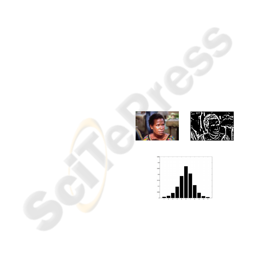
. Figure 1 illustrates the process of ob-

taining SH-features. Frames (a) and (b) show a color

image and its red channel response to a Laplacian ﬁl-

ter, respectively. The last panel shows the 11-bin his-

togram of the ﬁltered image.

(a) (b)

(c)

Figure 1: (a) An image; (b) the red-channel response to a

Laplacian ﬁlter; (c) the associated 11-bin histogram.

If F = {F

,.. . ,F

} is a bank of ﬁlters, the SH-

features associated with the family F is the collec-

tion h(I,F

), 1 6 i 6 r, combined into the single m-

dimensional vector

h(I, F) = (h(I,F

),. .. ,h(I,F

)), (2)

where m = rb. For a color image, m = 3rb. Banks of

ﬁlters used in this paper typically include Gabor ﬁlters

of different widths and orientations, gradient ﬁlters,

and Laplacian of Gaussians.

3 SH-FEATURES FOR

RETRIEVAL

To offer some evidence that SH-features are desirable

for image retrieval, we perform a preliminary retrieval

experiment using the Euclidean distance between his-

tograms. To be able to compare the results with those

reported in (Wang et al., 2001), we use the same sub-

set of the Corel data set consisting of 10 semantic cat-

egories, each with 100 images. We refer to this data

set as Corel-1000. The categories are listed in Table

1 and three samples from each category are shown

in Figure 2. As the examples suggest, even within a

semantic category, signiﬁcant variations are observed

among the images.

Table 1: Image categories in Corel-1000.

1 African People & Villages

2 Beach Scenes

3 Buildings

4 Buses

5 Dinosaurs

6 Elephants

7 Flowers

8 Horses

9 Mountains & Glaciers

10 Food

We utilize a bank of 5 ﬁlters and apply each ﬁl-

ter to the R, G, and B channels of the images to ob-

tain a total of 15 histograms per image. Each his-

togram consists of 11 bins so that the SH-feature vec-

tor h(I,F) has dimension 165. For a query image

I from the database, we calculate the Euclidean dis-

tances between h(I,F) and h(J,F), for every J in the

database, and rank the images according to increas-

ing distances. For comparison purposes, as in (Wang

et al., 2001), we calculate the weighted precision and

the average rank, which are deﬁned next. The re-

trieval precision for the top ℓ returns, is n

ℓ

/ℓ, where

ℓ

is the number of correct matches. The weighted

precision for a query image I is

p(I) =

100

∑

ℓ=1

ℓ

. (3)

For a query image I, rank order all 1,000 images in

the database, as described above. The average rank

r(I) is the mean value of the ranks of all images that

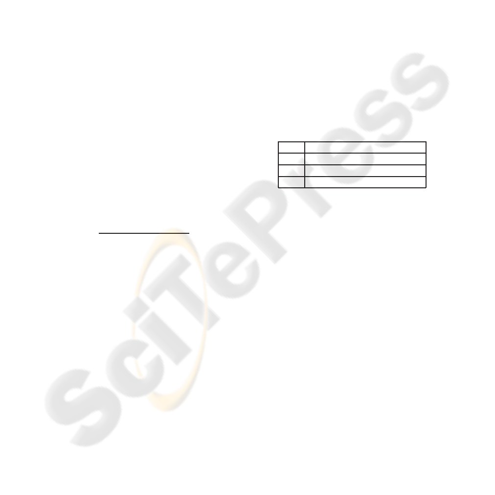
belong to the same class as I. Figures 3(a) and 3(b)

show the mean values

¯p

100

∑

I∈C

p(I) and ¯r

100

∑

I∈C

r(I), (4)

of the weighted precision and average rank within

each class C

, 1 6 i 6 10. High retrieval performance

is reﬂected in high mean precision and low mean rank.

Note that even without a learning component, the re-

sults obtained using SH-features and SIMPLIcity are

essentially comparable. Both perform considerably

better than color histograms with the earth mover’s

distance (EMD) investigated in (Rubner et al., 1997).

In Figure 3, color histograms 1 and 2 refer to EMD

applied to histograms with a different number of bins.

The results for SIMPLIcity and color histograms have

been reported in (Wang et al., 2001).

4 OPTIMAL FACTOR ANALYSIS

We introduce Optimal Factor Analysis (OFA), a lin-

ear feature learning technique whose goal is to ﬁnd

a linear mapping that reduces the dimension of the

data representation while optimizing the discrimina-

tive ability of the K-nearest neighbor (KNN) classi-

ﬁer as measured by its performance on given train-

ing data. We assume that a given ensemble of data

in Euclidean space R

is divided into training and

cross-validation sets, each consisting of labeled rep-

resentatives from P different classes of objects. For

an integer c, 1 ≤ c ≤ P, we denote by x

c,1

,.. .,x

c,t

and y

c,1

,.. . ,y

c,v

the training and cross-validation el-

ements that belong to class c.

If A: R

→ R

is a linear transformation, the

quantity

ρ(y

c,i

;A) =

min

c6=b, j

kAy

c,i

− Ax

b, j

min

kAy

c,i

− Ax

c, j

+ ε

(5)

provides a measurement of how well the nearest-

neighbor classiﬁer applied to the transformed data

identiﬁes the cross-validation element y

c,i

as belong-

ing to class c. Here, ε > 0 is a small number used

to prevent vanishing denominators and p > 0 is an

exponent that can be adjusted to regularize ρ in dif-

ferent ways. In this paper, we set p = 2. A large

value of ρ(y

c,i

;A) indicates that, after the transforma-

tion A is applied, y

c,i

lies much closer to a training

sample of the class it belongs to than to those of other

classes. A value ρ(y

c,i

;A) ≈ 1 indicates a transition

between correct and incorrect decisions by the near-

est neighbor classiﬁer. The special case of the func-

tion ρ, where p = 1, was used in the development of

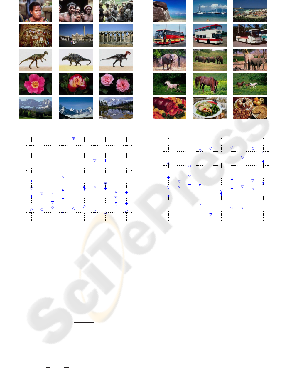
Figure 2: Samples from the dataset Corel-1000: three images from 10 classes, each consisting of 100 images.

1 2 3 4 5 6 7 8 9 10

0.1

0.2

0.3

0.4

0.5

0.6

0.7

0.8

0.9

Category ID

Average Precision

1 2 3 4 5 6 7 8 9 10

100

200

300

400

500

600

Category ID

Average Rank

Figure 3: (a) Plots of ¯p

and ¯r

, 1 6 i 6 10. The methods are labeled as follows: (▽) spectral histogram; (∗) SIMPLIcity; (◦)

color histogram 1; (+) color histogram 2.

Optimal Component Analysis (Liu et al., 2004). Note

that expression (5) can be easily modiﬁed to reﬂect

the performance of the KNN classiﬁer.

The idea is to choose a transformation A that max-

imizes the average value of ρ(y

c,i

;A) over the cross-

validation set. To control bias with respect to partic-

ular classes, we scale ρ(y

c,i

;A) with a sigmoid of the

form

σ(x) =

1+ e

−βx

(6)

before taking the average. We identify linear maps

A: R

→ R

with k × m matrices, in the usual way,

and deﬁne a performance function F : R

k×m

→ R by

F(A) =

∑

c=1

∑

i=1

σ(ρ(y

c,i

;A) − 1)

. (7)

Scaling an entire dataset does not change deci-

sions based on the nearest-neighbor classiﬁer. This is

reﬂected in the fact that F is (nearly) scale invariant;

that is, F(A) ≈ F(rA), for r > 0. Equality does not

hold exactly if ε 6= 0, but in practice, ε is negligible.

Thus, we ﬁx the scale and optimize F over matrices A

of unit Frobenius norm. Let

S =

A ∈ R

k×m

: kAk

= tr(AA

) = 1

(8)

be the unit sphere in R

k×m

. The goal of OFA is to

maximize the performance function F over S; that is,

to ﬁnd

A = argmax

A∈S

F(A). (9)

Due to the existence of multiple local maxima of F,

the numerical estimation of

A is carried out with a

stochastic gradient search. We omit the details since

the optimization strategy is similar to that employed

in (Liu et al., 2004), but much simpler because the

search is performed over a sphere instead of a Grass-

mann manifold.

4.1 An Interpretation of OFA

We interpret the dimension reduction via a linear map

A: R

→ R

and the Euclidean metric in the reduced

space in terms of the original m-dimensional features.

If A is a rank r matrix, take a singular value decom-

position

A = UΣV

, (10)

where U and V are orthogonal matrices of dimen-

sions k and m, respectively, and Σ is a k × m matrix

whose r× r northwest quadrant is diagonal with posi-

tive eigenvalues and whose remaining entries are all

zero. Let H be the r-dimensional subspace of R

spanned by the ﬁrst r columns of V and denote the

orthogonal projection of a vector x ∈ R

onto H by

. Then,

Ax· Ay = y

A)x = y

Kx = y

, (11)

for any x, y ∈ R

, where K = A

A is a positive semi-

deﬁnite symmetric matrix. In particular,

kAx− Ayk

= (x

− y

)

K(x

− y

). (12)

This means that the Euclidean distance between fea-

ture vectors in the reduced space R

can be interpreted

as the distance between the projected vectors x

and

in the original feature space with respect to the

new metric

d(x

) =

− y

)

K(x

− y

). (13)

Note that the subspace H is spanned by the eigenvec-

tors of K associated with its non-zero eigenvalues, so

that (13) does deﬁne a metric on H. Thus, OFA can

be viewed as a technique to learn from a training set

an optimal subspace of the feature space R

for di-

mension reduction and an inner product whose asso-

ciated metric is optimal for categorization based on

the nearest-neighbor classiﬁer.

4.2 A Leave-One-Out Strategy

In applications of OFA to image retrieval, or in sit-

uations where the training set is not very large, a

leave-one-out strategy is adopted during the optimiza-

tion process. In other words, for a candidate linear

map A, the value F(A) of the performance function

is replaced with the average value of F over several

passes, as follows. In each pass, the cross-validation

set consists of a single element taken from the train-

ing set and F(A) is calculated according to (7). Then,

the average value over the entire training set is used

to quantify performance in the optimization process.

5 IMAGE CATEGORIZATION

We report the results of several image categorization

experiments with the Corel-1000 data set described

in Section 3. In each experiment, we placed an equal

number of images from each class in the training set

and used the remaining ones as query images to be

indexed by the nearest neighbor classiﬁer applied to

a reduced feature learned with OFA. Initially, an im-

age is represented by an SH-feature vector h(I,F) of

dimension 165 obtained from the 11-bin histograms

associated with 5 ﬁlters applied to the R, G, and B

channels; OFA was used to reduce the dimension to

k = 9. Table 2 shows the categorization performance:

T denotes the total number of images in the training

set, and categorization performance refers to the rate

of correct indexing using all 1,000− T images out-

side the training set as queries.

Table 2: Results of categorization experiments with the

Corel-1000 data set. T is the number of training images

and the dimension of the reduced feature space is 9.

T Categorization Performance

600 84.5%

400 84.3%

200 73.9%

6 IMAGE RETRIEVAL

We now use the classiﬁer learned for content-based

image categorization to retrieve images according to

their contents. We begin with the remark that the clas-

siﬁer was optimized to categorize query images cor-

rectly according to the nearest neighbor criterion, but

not necessarily to rank matches to a query image cor-

rectly according to distances in feature space. Thus,

in contrast with the retrieval strategy based solely on

distances adopted, e.g., in (Wang et al., 2001) and

(Hoi et al., 2006), we propose to exploit the strengths

of the image categorization classiﬁer in a more essen-

tial way.

Let A: R

→ R

be the optimal linear dimension-

reduction map learned with OFA. If I is an image and

h(I, F) ∈ R

is the associated SH-feature vector, we

let x denote its projection to R

; that is,

x = Ah(I,F). (14)

If there are P classes of images, for each i, 1 6 i 6

P, let x

be the reduced feature vector of the training

image in class i, which is closest to x. To each i, we

assign a probability p(i|I) that I belongs to class i, as

1 2 3 4 5 6 7 8 9 10

0.2

0.3

0.4

0.5

0.6

0.7

0.8

0.9

Category ID

Average Precision

1 2 3 4 5 6 7 8 9 10

100

150

200

250

300

350

Category ID

Average Rank

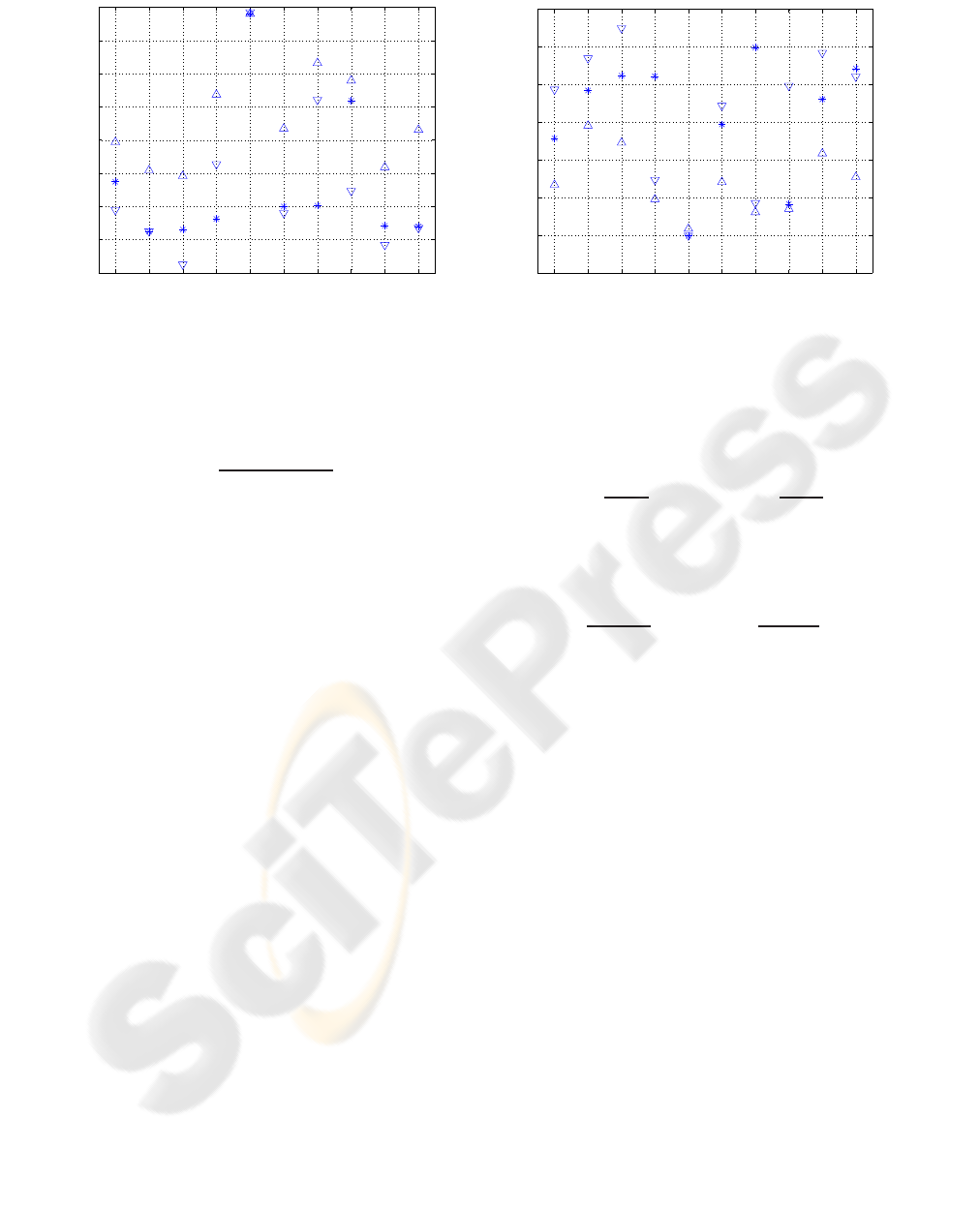
(a) (b)

Figure 4: (a) Average precision within each class; (b) average rank. The methods are labeled as follows: (▽) spectral

histogram; (∗) SIMPLIcity; (△) OFA-400.

follows:

p(i|I) =

−kx−x

∑

j= 1

−kx−x

. (15)

Given a query image I and a positive integer ℓ, the

goal is to retrieve a ranked list of ℓ images from the

database. We assume that all images in the database

havebeen indexedaccordingto content using the clas-

siﬁer learned with OFA. Rank the classes according

to the probabilities p(i|I). We retrieve images as fol-

lows: select as many images as possible from the most

likely class; once that class is exhausted, we proceed

similarly with the second most likely class and iter-

ate the procedure until ℓ images are obtained. Within

each class, the images are retrieved and ranked ac-

cording to their Euclidean distances to I as measured

in the reduced feature space.

6.1 Experimental Results

We report the results of retrieval experiments with the

Corel-1000 dataset. To quantify performance in an

objective manner, we only use query images that are

part of the database. Since each class contains 100

images, the maximum possible number of matches to

a query image is 100, where a match is an image that

belongs to the same class. We ﬁrst compare retrieval

results using OFA learning with those obtained with

SIMPLIcity and spectral histograms, as described in

Section 3. We calculated the mean values ¯p

and ¯r

the weighted precision and rank as deﬁned in (4). The

plots shown in Figure 4 show a signiﬁcant improve-

ment in retrieval performance with a learning compo-

nent. OFA was used with 400 training images.

We further quantify retrieval performance, as fol-

lows. For an image I and a positive integer ℓ, let m

ℓ

be the number of matching images among the top ℓ

returns. Deﬁne

ℓ

(I) =

ℓ

(I)

ℓ

and r

ℓ

(I) =

ℓ

(I)

100

, (16)

which are the precision and recall rates for ℓ returns

for image I. The average precision and average recall

for the top ℓ returns are deﬁned as

ℓ

∑

ℓ

(I)

1000

and r

ℓ

∑

ℓ

(I)

1000

, (17)

respectively. Here, the sum is taken over all 1,000 im-

ages in the database. Note that, for a perfect retrieval

system, p

ℓ

= 1, for 1 6 ℓ 6 100, and gradually decays

to p

1000

= 0.1; similarly r

ℓ

= 1, for ℓ ≥ 100 decaying

to r

= 0.01.

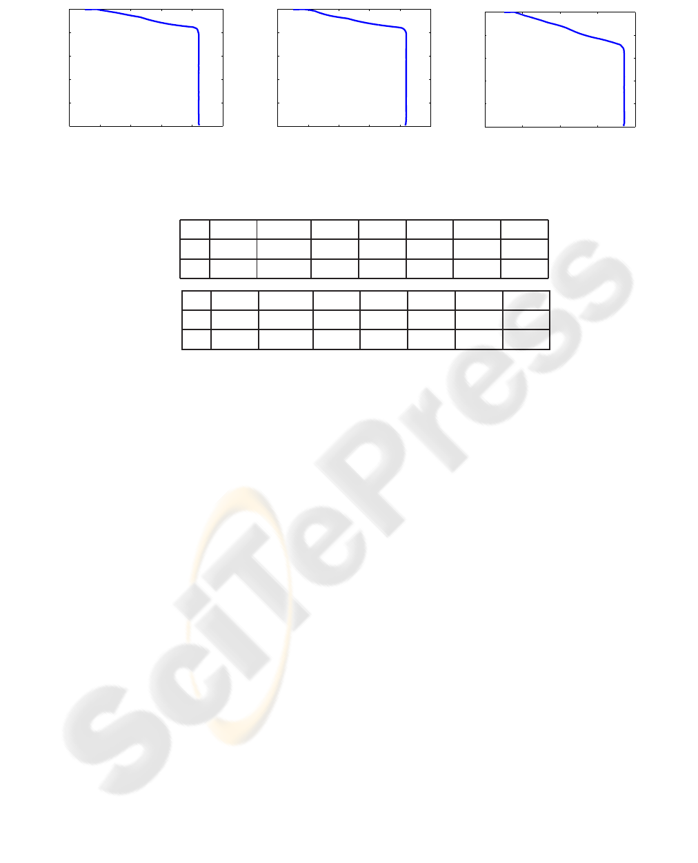
Table 3 shows several values of the average pre-

cision and average recall based on a 9-dimensional

classiﬁer learned with T training images. The full

average-precision-recall plots are shown in Figure 5.

Figure 6 shows the top 10 returns for a few images

in the database for a classiﬁer trained with T = 400

images. In each group, the ﬁrst image is the query

image, which is also the top return.

7 CONCLUSION

We represented images using histograms of their

spectral components for content-based image cate-

gorization and retrieval. A learning technique was

developed to reduce the dimension of the represen-

tation and optimize the discriminative ability of the

nearest-neighbor classiﬁer. Several experiments were

carried out and the results indicate a very signiﬁcant

improvement in retrieval performance over a number

0 0.2 0.4 0.6 0.8 1

0.2

0.4

0.6

0.8

Precision

Recall

0 0.2 0.4 0.6 0.8 1

0.2

0.4

0.6

0.8

Precision

Recall

0 0.2 0.4 0.6 0.8

0.2

0.4

0.6

0.8

Precision

Recall

Figure 5: Corel-1000: plots of the average-precision × average-recall for 600, 400, and 200 training images.

Table 3: Retrieval results with T training images. Average retrieval precision (p

ℓ

) and recall (r

ℓ

) for the top ℓ matches.

T = 600

ℓ 10 20 40 70 100 200 500

ℓ

0.842 0.0842 0.843 0.843 0.832 0.466 0.198

ℓ

0.084 0.168 0.337 0.590 0.832 0.930 0.992

T = 400

ℓ 10 20 40 70 100 200 500

ℓ

0.840 0.0840 0.840 0.841 0.828 0.460 0.199

ℓ

0.084 0.168 0.336 0.589 0.828 0.919 0.996

of existing retrieval systems. Reﬁnements to obtain

sparse representations and incorporate kernel tech-

niques to cope with nonlinearity in data geometry, re-

trieval strategies for real-time execution, as well as a

user feedback component will be investigated in fu-

ture work.

ACKNOWLEDGEMENTS

This work was supported in part by NSF grants CCF-

0514743 and IIS-0307998, and ARO grant W911NF-

04-01-0268.

REFERENCES

Carson, C., Thomas, M., Belongie, S., Hellerstein, J., and

Malik, J. (1999). Blobworld: a system for region-

based image indexing and retrieval. In Proc. Visual

Information Systems, pages 509–516.

Hoi, S., Liu, W., Lyu, M., and Ma, W.-Y. (2006). Learning

distance metrics with contextual constraints for image

retrieval. In Proc. CVPR 2006.

Liu, X. and Mio, W. (2006). Splitting factor analysis and

multi-class boosting. In Proc. ICIP 2006.

Liu, X., Srivastava, A., and Gallivan, K. (2004). Optimal

linear representations of images for object recogni-

tion. IEEE Trans. Pattern Analysis and Machine In-

telligence, 26:662–666.

Portilla, J. and Simoncelli, E. (2000). A parametric texture

model based on joint statistics of complex wavelet co-

eﬁcients. International Journal of Computer Vision,

40:49–70.

Rubner, Y., Guibas, L., and Tomasi, C. (1997). The

earth mover’s distance, multi-dimensional scaling,

and color-based image databases. In Proc. DARPA Im-

age Understanding Workshop, pages 661–668.

Smith, J. and Li, C. (1999). Image classiﬁcation and query-

ing using composite region templates. Computer Vi-

sion and Image Understanding, 75(9):165–174.

Wang, J., Li, J., and Wiederhold, G. (2001). SIMPLIcity:

Semantics-sensitive integrated matching for picture li-

braries. IEEE Trans. on Pattern Analysis and Machine

Intelligence, 23(9):947–963.

Wu, Y., Zhu, S., and Liu, X. (2000). Equivalence of Julesz

ensembles and FRAME models. International Jour-

nal of Computer Vision, 38:247–265.

Yin, P.-Y., Bhanu, B., Chang, K.-C., and Dong, A. (2005).

Integrating relevance feedback techniques for im-

age retrieval using reinforcement learning. IEEE

Trans. on Pattern Analysis and Machine Intelligence,

27(10):1536–1551.

Zhu, S., Wu, Y., and Mumford, D. (1998). Filters, random

ﬁelds and maximum entropy (FRAME). International

Journal of Computer Vision, 27:1–20.

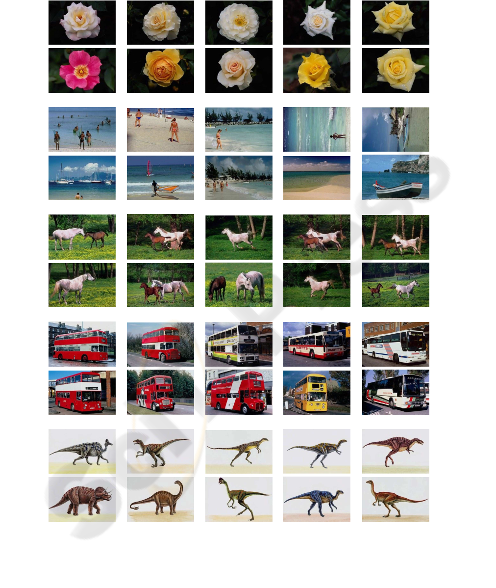
(a)

(b)

(c)

(d)

(e)

Figure 6: Examples of top ten returns. In each group, the ﬁrst image is the query, which is also the top return.