
MRI SEGMENTATION USING MULTIFRACTAL ANALYSIS
AND MRF MODELS
Su Ruan
CReSTIC, Dept GEII, IUT de Troyes, 10026 Troyes Cedex, France
Jonathan Bailleul
GREYC, ENSICAEN, 6 Bd. Maréchal Juin, 14050 Caen Cedex, France
Keywords: Multifractal analysis, Markov Random Field, image segmentation, Magnetic Resonance Imaging.
Abstract: In this paper, we demonstrate the interest of the multifractal analysis for removing the ambiguities due to
the intensity overlap, and we propose a brain tissue segmentation method from Magnetic Resonance
Imaging (MRI) images, which is based on Markov Random Field (MRF) models. The brain tissue
segmentation consists in separating the encephalon into the three main brain tissues: grey matter, white
matter and cerebrospinal fluid (CSF). The classical MRF model uses the intensity and the neighbourhood
information, which is not robust enough to solve problems, such as partial volume effects. Therefore, we
propose to use the multifractal analysis, which can provide information on the intensity variations of brain
tissues. This knowledge is modelled and then incorporated into a MRF model. This technique has been
successfully applied to real MRI images. The contribution of the multifractal analysis is proved by
comparison with a classical MRF segmentation using simulated data.
1 INTRODUCTION
Image segmentation is a classical problem in
computer vision and of paramount importance to
medical imaging. Proper tissue classification
enables: a) quantitative volumetric analysis on
various brain structures; b) morphological analysis
to assess intracranial deformation caused by brain
tumours; c) visualisation for surgical planning and
guidance.
In this paper, we deal with tissue segmentation of
Magnetic Resonance Imaging (MRI) brain images.
Numerous semi-automatic and automatic
segmentation techniques have already been
developed to replace manual segmentation which is
a labour-intensive, subjective and thereby non
reproducible procedure. Actually, the main
techniques are based on: texture analysis
(Schad,1993), histogram threshold determination
(Suzuki, 1991), cluster analysis (Simmons, 1994)
and fuzzy cluster analysis (Pham, 1999), a priori
information about anatomy (Joliot, 1993), or MRF
segmentation (Held, 1997)(Choi, 1997). Although
there exists many image classification algorithms,
the methods usually suffer from the fact that in
practice there is a significant overlap in intensity
values between tissue types, owing to magnetic field
inhomogeneity, susceptibility artefacts and partial
volume effects (one pixel mixed of two or more than
two classes). Our idea, about this issue, is to
describe the brain tissue using the relative intensity
variations, rather than using only absolute intensity
values. The multifractal analysis is adopted here to
this objective. It was first introduced in the context
of turbulence, and then studied as a mathematical
tool as well as in many applications such as image
processing (Sarkar,1995) (Levy-Véhel, 1996)
(Grazzini, 2005). Due to the presence of noise in
MRI images, it is important to take into account
contextual information. This can be done a priori
using MRF models which are appropriate to specify
spatial dependencies by a priori label field
distribution (Geman, 1984) (Choi,1997).
In this paper, we demonstrate the interest of the
multifractal analysis to remove the ambiguities due
to the intensity overlap and propose a tissue
segmentation method based on Markov Random
101
Ruan S. and Bailleul J. (2007).
MRI SEGMENTATION USING MULTIFRACTAL ANALYSIS AND MRF MODELS.
In Proceedings of the Second International Conference on Computer Vision Theory and Applications, pages 101-106
DOI: 10.5220/0002046901010106
Copyright
c
SciTePress

Field (MRF) models. The brain segmentation
consists in separating the encephalon into the three
main brain tissues: grey matter, white matter and
CSF. The classical MRF model uses the intensity
and the neighbourhood information, but it is not
robust enough to solve the problems such as partial
volume effects. Therefore, we propose to
supplement the multifractal analysis to the classical
MRF model, which can provide the information
about intensity variations of the brain tissues.
2 MULTIFRACTAL ANALYSIS OF
IMAGES
It is well known that the geometrical complexity of a
“fractal” set may be described, in a global way, by
giving its dimension. In order to describe the local
singular behaviour of measures or signals, the
multifractal analysis is proposed to give either
geometrical or probabilistic information about the
distribution of points having the same singularity
(Levy-Véhel, 1996, 2000). The value of Hölder
exponent α is usually used to obtain a local
information about the pointwise regularity. The so-
called “multifractal spectrum” f(
α
) gives the
geometrical or probabilistic information. Some
spectra, such as Hausdorff spectrum f
h
and large
deviation spectrum f
g
, have been defined and studied
(Levy-Véhel,1998). The multifractal analysis of
images usually consists in computing values of
Hölder exponentα and its multifractal spectrum,
then classifying each point according both to the
value of Hölder exponent α and to the corresponding
spectrum f(
α
). In this paper, we are only interested
in the local information provided by the Hölder
exponent
α
.
2.1 The Hölder Exponent α
Let μ be a Borel probability measure laid upon a
compact set P. For each point x in P, the Hölder
exponent α can be defined as follows (Levy-Véhel,
1996)(Canus 1996) (more rigorous and complete
definitions are given in (Brown, 1992) (Levy-
Véhel,1998)):
δ
μ
α
δ
δ
log
))((log
lim)(
0
xB
x
→
= (1)
where
)(xB
δ
is an open-ball of diameter
σ
centred
on the point x. It reflects the local behaviour of the
measure
μ
around x. In image analysis, the points in
the equation (1) are naturally associated to the pixels
of the image, the open-balls to windows in 2D and
balls in 3D centred on each pixel, the measures to
functions of grey level intensities. In our case, the
measure
μ
is defined as the sum of the grey level
intensities of pixels within a neighbourhood V
(δ)
defined by a ball of diameters
σ
The Hölder
exponent α can be assessed as the slope of
log[
μ
(V(
δ
))] versus log
δ
.
δ
changes linearly from 1
to the maximum value with unity step. If the
maximum diameter of the neighbourhood is chosen
small, α reacts to localize singularities. If the
maximum diameter is large, α reacts to more
widespread singularities. Thanks to the choice of the
measure function
μ
(V(
δ
)), we can obtain the
following local information via the Hölder exponent:
let us note α0 the Hölder exponent within a intensity
uniform (homogeneous) region. If the value of
α
for
the current pixel is higher than
α
0, it is surely within
a intensity concave region (valley), while in the
inverse case, the current voxel is in a intensity
convex region (hill). The illustration of the different
values of α is shown in Figure 1. In fact,
μ
(V(
δ
)) in a
concave region increases more rapidly in function of
V(
δ
) than that in a convex region. The value α0 lies
between them.
0
α
α
=
0
α
α
>
0
α
α
<
Figure 1: Illustration of α for different spatial variations of
intensity.
2.2 MRI Images
The local image information provided by α is very
helpful in the situation of low contrast, since it can
discriminate the three situations described above. As
known, the cortex of the brain has many
circumvolutions. Thus, it leads to intensity
variations in image, which can be easily described
by the multifractal analysis. In MRI images, the
sulcus can be considered as a valley in term of
intensity, and the CSF is generally at the bottom of
the valley. On the contrary, the gyrus can be
considered as a hill, and the white matter,
surrounded by the grey matter, is at the top of the
hill. The problems of the partial volume effects and
of the low contrast are essentially present in these
two types of regions. Most of the homogeneous
regions can be found within the white matter (in the
VISAPP 2007 - International Conference on Computer Vision Theory and Applications
102
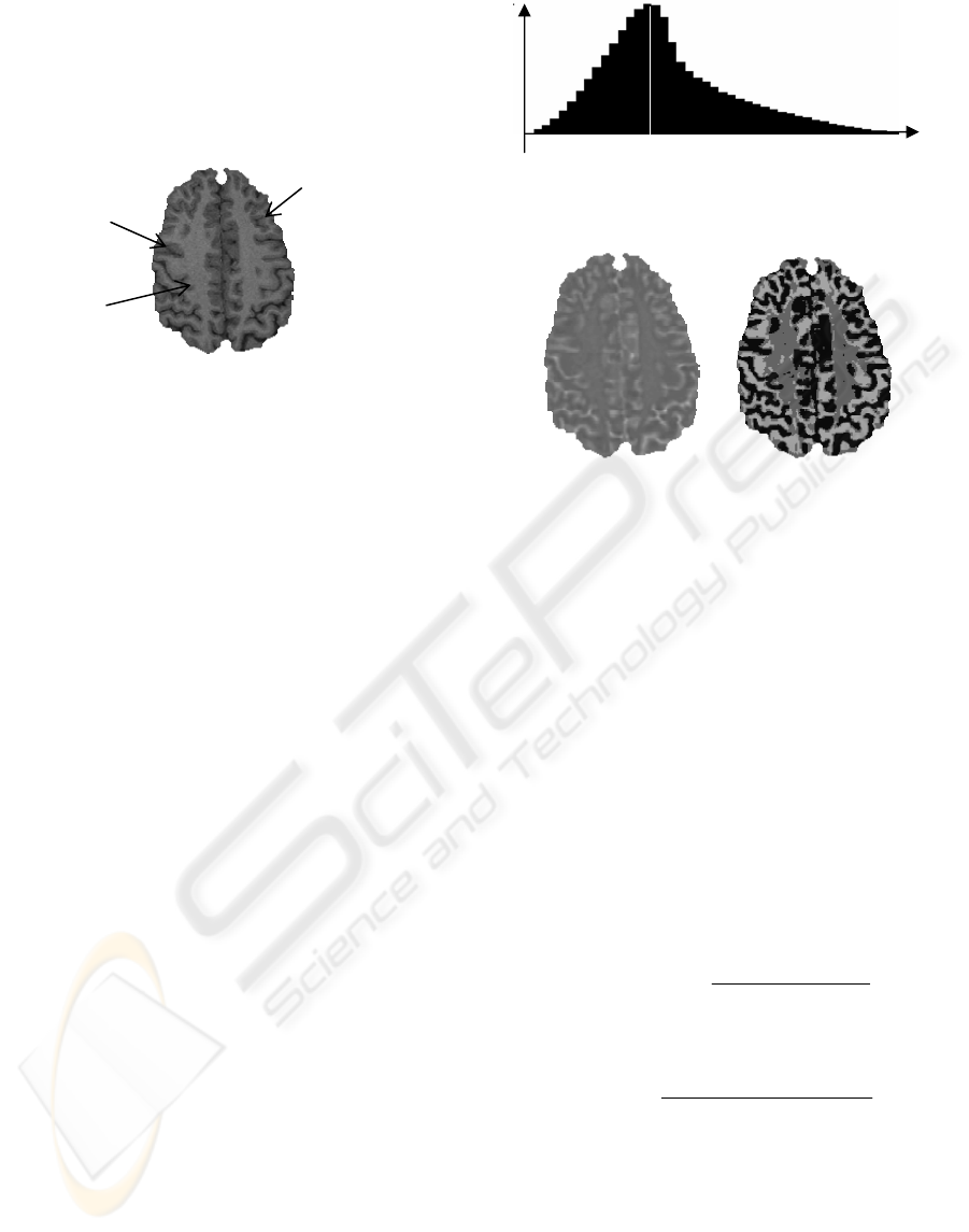
center of the brain) and a few others within the grey
matter. The Figure 2 shows one axial MRI slice in
which examples of the three types of region are
pointed out.
Figure 2: Three regions in MRI data: convex, concave and
homogeneous region
.
The difficulties of the segmentation are mainly
founded in the regions of the gyri and sulci due to
the partial volume effects. The a priori knowledge
about these two regions described by the Hölder
exponent
α
can help us to cope with this problem.
The histogram of
α
obtained from a T1-wheighted
MRI data set (256×256×124 pixels, with a resolution
of 0.9375×0.9375×1.2mm³) is shown in Figure 3. Its
form is always concave for the MRI data, because of
the brain morphology. In fact, the area of the
homogeneous region, usually in white matter, is
larger than that of the others regions (concave and
convex regions). Therefore,
α
0
describing an
homogeneous region, can be easily found by
detecting the peak of the histogram. Since we are
just interested in three types of region (concave,
homogeneous and convex), and do not pay attention
to the degree of concavity or convexity, we can
define a function f(
α
) as follows to obtain the three
types of region :
⎪
⎩
⎪
⎨
⎧
>−
=
<
=
0
0
0
)( 1
)( 0
)( 1
)(
αα
αα
αα
α
x if
x if
xif
f
(2)
Figure 4 shows one
α
slice (the original image is
shown in Figure 2) and the three types of region
obtained using (2) : concave, convex and
homogeneous regions. The measure region is a cube
of 3×3×3 pixels. The value of
α
0, found from the
peak of the histogram of
α
is 2.29. Comparing to the
original image, it can be observed that the
homogeneous regions correspond mainly to the
white matter, and the values of
α
correctly reflect
the hills and valleys in the image.
Figure 3: Histogram of α calculated from a 3D MRI
volume. The measure region is 3x3x3 voxels.
Figure 4: One slice of α image (left) and the three types of
region (right): convex region in deep grey colour, concave
region in white colour and homogeneous in light grey
colour.
3 MARKOVIAN
SEGMENTATION
We propose to incorporate a priori information about
multifractal characterisation into the MRF model.
Let us consider three random fields: Y={Ys, s
∈
S}
represents the field of observations located on a
lattice S of N sites s, X={Xs, s
∈
S} the label field and
A={
α
s, s
∈
S} the multifractal field. Each Ys takes its
value in
Λ
obs
={0…,255}, each Xs in {1=CSF, 2=gray
matter, 3=white matter} and each
Α
s in {-1,0,1
}
(see
equation (2)). We use the Bayes rule to write:
),(
)()/,(
),/(
ss
ssss
sss
yP
xPxyP
yxP
α
α
α
= (3)
Since the two fields Ys and As are independent, (3)
becomes:
),(
)()/()/(
),/(
ss
sssss
sss
yP
xPxPxyP
yxP
α
α
α
= (4)
We look for the x
s
that maximises the left-hand side
of (4). Since
),(
ss
yP
α
does not depend on the x
s
,
this is equivalent to write:
)()/()/(maxarg
ˆ
sssss
s
s
xPxPxyP
x
x
α
=
(5)
Sulcus :
Convex region
White matter :
homogeneous
re
g
ion
Gyrus:
concave region
α
α
0
MRI SEGMENTATION USING MULTIFRACTAL ANALYSIS AND MRF MODELS
103

In accordance with the Hammersley and Clifford
theorem (Geman, 1984),
)( sxP
is defined by a
Gibbs distribution,
))(exp(
1
)(
2 ss
xU
Z
xP −≡
(6)
where U2 stands for the energy function and Z is a
normalising constant.
Denoting
))/(exp(
'
1
)/( 1 ssss xyU
Z
xyP −= and
))/(exp(
''
1
)/(
3 ssss
xU
Z
xP
αα
−= , Eq.(6) can be
defined in terms of an energy function that has to be
minimised:
{}
)7()/()()/(minarg
ˆ
321 sssss
x
s
xUxUxyUx
x
α
+
+
=
Let us consider the terms U1. In MRI data, the
distribution of the grey levels of each tissue has
a gaussian form, and there is no correlation
between them. The data energy term is thus
expressed as :
)2ln(
2
)(
)/(
2
2
1
s
s
s
x
x
xs
ss
my
xyU
σπ
σ
+
−
= (8)
Let’s consider now U
2
(x
s
), the energy term
corresponding to the a priori model. We adopt a
3D system of second-order neighbourhood C,
consisting of the 18 nearest neighbours. Using
standard isotropic Potts model, one obtains :
)),(1()(
,
2 t
Cts
ss
xxxU
∑
∈
−−=
δβ
(9)
where
β
is a weight coefficient, and is the Kronecker
delta function. U
2
is minimum for a homogeneous
region.
The energy term U3
(α
s
/ x
s
) is defined in order to
advantage the choice of the CSF label or white
matter label for a site whether it is in a convex
region or a concave region respectively. Since
only two types of region are interesting in our
case, U3
(α
s
/ x
s
) can be defined according to
f(
α
). It becomes :
⎪
⎩
⎪
⎨
⎧
=−
=
=
otherwise 0
3 if
1 if
)()/(
3 sconcave
sconvex
sss
xκ
xκ
fxU
αα
(10)
where
convexconcave
κ
κ
and are constant (>0).
If one pixel has a grey level near the middle of
the means of the CSF and the gray matter or the
middle of the means of the grey matter and the white
matter, its U
1
is not dominant. The classification of
this pixel depends mainly on the U
2
and U
3
terms.
Therefore, the a priori information brought by U
3
is
very useful in this case.
We use the deterministic relaxation algorithm
ICM (Besag, 1974) to minimise the global energy
function U. For the initialisation, we exploit a
maximum likelihood segmentation depending only
on U
1
.
4 RESULTS
In order to show the improvement of the
segmentation by addition of the multifractal term
U3, simulated MRI data were used, which are
available on the site BrainWeb (Collins,1998). This
three-dimensional phantom is made up of ten
volumetric data sets that define the spatial
distribution of different tissues (e.g. grey matter,
white matter, CSF, etc), where the voxel intensity is
proportional to the fraction of tissue within the
voxel. A threshold value equal to 50% can be used
to obtain the voxels belonging to the corresponding
tissue, which is considered as the gold standard.
Each volume data consists of 181×217×181 voxels,
whose size is 1×1×1mm3. The simulated MRI
volume with a noise level of 7% is used for our
study. It was firstly segmented by the software
developed in our laboratory (Moretti, 2000) to
obtain the encephalon in which there are only the
three brain tissues (Figure 5).
The segmentation results are evaluated by
measuring the sum, denoted
total
ξ
, of the false
positive ratio
fp
ξ
and the false negative ratio
fn
ξ
.
fp
ξ
is defined as the number of misclassified voxels
divided by the number of good voxels taken from
the gold standard (N). The false negative ratio
fn
ξ
is
defined as the number of lost good voxels divided by
N.
In order to obtain the initial values of the means
and the variances used in U
1
(y
s
/x
s
) to carry out the
initialisation of the segmentation, we used the
Davidon-Fletcher-Powell method described in
(Press, 1992) to fit the intensity histogram of the
encephalon data set by a sum of three gaussian
functions. Since the phantom is relatively realistic,
studies on the choice of the parameters used in the
models were carried out. The parameters β and κ can
be chosen in the ranges
]5.0 ,1.0[
∈
β
and ]5.1 ,5.0[∈
κ
which provide acceptable
total
ξ
. According to our
experience, the algorithm ICM is not very sensitive
to the value βbut rather to the initialisation of the
VISAPP 2007 - International Conference on Computer Vision Theory and Applications
104
segmentation. To reduce this dependence on the
initialisation, the means and variances are re-
estimated at each iteration. A comparison of the
results obtained by the classical Markovian
segmentation and the proposed segmentation method
is performed and shown in Table 1 (β =0.2, κ
convex
=
κ
concave
=1.1). We can observe that the total error
total
ξ
on each tissue is reduced using the function U
3
in addition. As discussed above, the a priori
information modelled by U
3
can ameliorate the
results in the case of low contrast. These cases are
usually apparent in the boundaries of tissues or in
gyri and sulci, which represent a small percentage of
total volume data. That is why the improvement is
about 2%. The errors for the CSF segmentation seem
to be more than those for the others. That is because
the number of CSF voxel is much lower than those
of the other tissues, thus it easily results a high
relative error ratio.
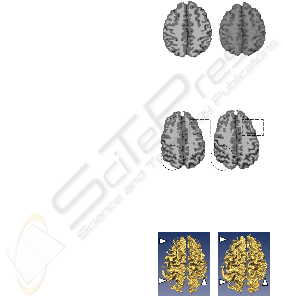
Real MRI data were also used to evaluate
visually the results. The corresponding result of the
image shown in Figure 2 is illustrated in Figure 6.
Compared to the classical Markovian segmentation,
the segmentation integrating the multifractal
information favours the sulci and gyri if the contrast,
due to the partial volume effects, is low in these
regions. Two small windows are located in Figure 6
to show the amelioration in critical regions. The
discontinuities of the white matter and sulci obtained
by the classical MRF segmentation are significantly
repaired by the proposed method. To illustrate more
clearly this issue, volume-rendered images of the
white matter are used (Figure 7). As known, the
white matter of the human is a continuously
connected structure, thus the volume-rendered image
using the proposed method depicts more accurately
the white matter.
5 CONCLUSION
We have presented a MRF segmentation method
incorporating the a priori multifractal information
model, aiming to segment MRI brain tissues. The
Hölder exponent α permits to describe locally the
intensity variations, therefore helping to remove the
ambiguities due to the low contrast and the partial
volume effects. Three types of region: concave,
convex and homogeneous region are used in our
model. The results obtained on the digital phantom
and the real MRI data show quantitatively and
qualitatively improvement of the brain
segmentation.
Although the empirical values, chosen for the
model parameters (
β
,
κ
convex
and
κ
concave
), give
satisfying results, adapted values to different volume
data will be more efficient and make the
segmentation more accurate. The estimation of these
hyperparameters is an important issue in the future
work.
Figure 5: One slice of gold standard (left) and the
corresponding slice of the simulated data with a level
noise of 7% (right). The three tissues are colour-coded as
follows: white matter =white colour, grey matter =grey
colour, CSF =black.
Figure 6: Comparison of results of the slice shown in
Figure 2 with (right) and without (left) use of the
multifractal analysis. Three tissues are obtained: white
matter (white colour), grey matter (grey colour) and CSF
(black). The improvements can be observed in the circle
windows concerning the white matter and the rectangular
windows concerning the CSF.
Figure 7: Volume-rendered images of the white matter
obtained from the classical MRF segmentation (left) and
the proposed segmentation method (right). Some
discontinuities of structures (left) and improvements
(right) are pointed out by arrows.
MRI SEGMENTATION USING MULTIFRACTAL ANALYSIS AND MRF MODELS
105

Table 1: Comparison of the results obtained by the
classical MRF segmentation (Method 1) and by the
proposed method (Method 2), using the false positive ratio
fp
ξ
and the false negative ratio
fn
ξ
.
Method 1 (%) Method 1 (%)
Tissue
fp
ξ
fn
ξ
total
ξ
%)
fp
ξ
fn
ξ
total
ξ
WM 3.12 8.50 11.62 3.88 5.87 9.7
GM 7.99 5.02 13.01 6.19 5.09 11.2
CSF 13.37 7.78 21.15 10.76 8.78 19.
REFERENCES
Besag, J., 1974. On the statistical analysis of dirty
pictures. J.R. Statist. Soc. B-48, 259-302.
Brown, G., Michon, G. and Peyrière, J., 1992. On the
Multifractal analysis of measures. J.Stat. Phys. 66,
775-790.
Canus, C., Lévy-Véhel, J., 1996. Change detection in
sequences of images by multifractal analysis. Proc. of
ICASSP'96, May 7-10, Atlanta.
Choi, S. M., Lee, J. E. and Kim, M. H., 1997. Volumetric
object reconstruction using the 3D-MRF model-based
segmentation, IEEE. Trans. Med. Imag.16, 887-892.
Collins, D.L. and al., 1998. Design and construction of a
realistic digital brain phantom. IEEE. Trans. Med.
Imag.,17, 463-468 (http: //www.bic.mni.mcgill.ca
/brainweb).
Geman, S. and Geman, D., 1984. Stochastic relaxation,
Gibbs distribution, and the Bayesian restoration of
images. IEEE Trans. Pattern Analysis and Machine
Intelligence 6, 721-741.
Grazzini, J., Turiel, A., Yahia, H., 2005. Presegmentation
of high-resolution satellite images with a multifractal
reconstruction scheme based on an entropy criterium.
Proceeding of IEEE ICIP-2005, Volume: 1, On
page(s): I- 649-52.
Held, K., Kops, E. R., Krause, B. J., Wells, W. M.,
Kikinis, R. and Müller-Gärtner, H. W., 1997. Markov
Random Field segmentation of brain MR images,
IEEE. Trans. on Med. Imag. 16, 878-892.
Joliot, M. and Mazoyer, B., 1993. Three-dimensional
segmentation and interpolation of magnetic resonance
brain images. IEEE Trans. Med. Imag.12, 269-277.
Levy-Véhel, J., 1996. Introduction to the multifractal
analysis of images. In Fractal Encoding and analysis.
Yuval Fisher Editor, Springer Verlag.
Levy-Véhel, J., Vojak, R., 1998. Multifractal analysis of
choquet capacities: preliminary results. Adv.in Appl.
Math. 20, 1-43.
Levy-Véhel, J., 2000. Signal enhancement based on
Hölder regularity analysis. In IMA Volumes in
Mathematics and its Applications, Volume 132, pp.
197-209.
Moretti, B., Fadili, J., Ruan, S., Bloyet, D. and Mazoyer,
B., 2000. Phantom-based performance evaluation-
application to brain segmentation from magnetic
resonance images. Medical Image Analysis, Vol. 4,
No. 4, pp. 303-316, June, 2000.
VISAPP 2007 - International Conference on Computer Vision Theory and Applications
106
