COMBINATION OF VIDEO-BASED CAMERA TRACKERS USING

A DYNAMICALLY ADAPTED PARTICLE FILTER

David Marimon and Touradj Ebrahimi

Signal Processing Institute

Swiss Federal Institute of Technology (EPFL)

Lausanne, Switzerland

Keywords:

Sensor fusion, video camera tracking, particle ﬁlter, adaptive estimation.

Abstract:

This paper presents a video-based camera tracker that combines marker-based and feature point-based cues in

a particle ﬁlter framework. The framework relies on their complementary performance. Marker-based trackers

can robustly recover camera position and orientation when a reference (marker) is available, but fail once the

reference becomes unavailable. On the other hand, feature point tracking can still provide estimates given a

limited number of feature points. However, these tend to drift and usually fail to recover when the reference

reappears. Therefore, we propose a combination where the estimate of the ﬁlter is updated from the individual

measurements of each cue. More precisely, the marker-based cue is selected when the marker is available

whereas the feature point-based cue is selected otherwise. The feature points tracked are the corners of the

marker. Evaluations on real cases show that the fusion of these two approaches outperforms the individual

tracking results.

Filtering techniques often suffer from the difﬁculty of modeling the motion with precision. A second related

topic presented is an adaptation method for the particle ﬁler. It achieves tolerance to fast motion manoeuvres.

1 INTRODUCTION

Combination of tracking techniques has proven to be

necessary for some camera tracking applications. To

reach a synergy, techniques with complementary per-

formance have ﬁrst to be identiﬁed. Research on cam-

era tracking has concentrated on combining sensors

within different modalities (e.g. inertial, acoustic, op-

tic). However, this identiﬁcation is possible within

a single modality: video trackers. Video-based cam-

era tracking can be classiﬁed into two categories that

have compensated weaknesses and strengths: bottom-

up and top-down approaches (Okuma et al., 2003).

For the ﬁrst category, the six Degrees of Freedom

(DoF), 3D position and 3D orientation, estimates are

obtained from low-level 2D features and their 3D geo-

metric relation (such as homography, epipolar geom-

etry, CAD models or patterns), whereas for the sec-

ond group, the 6D estimate is obtained from top-down

state space approaches using motion models and pre-

diction. Marker-based systems (Zhang et al., 2002)

can be classiﬁed in the ﬁrst group. Although they

have a high detection rate and estimation speed, they

still lack tracking robustness: the marker(s) must be

always visible thus limiting the user actions. In con-

trast to bottom-up approaches, top-down techniques

such as ﬁlter-based camera tracking allow track con-

tinuation when the reference is temporarily unavail-

able (e.g. due to occlusions). They use predictive

motion models and update them when the reference

is again visible (Davison, 2003; Koller et al., 1997;

Pupilli and Calway, 2005). Their weakness is, in gen-

eral, the drift during the absence of a stable reference

(usually due to feature points difﬁcult to recognise af-

ter perspective distortions).

Filtering techniques often suffer from the difﬁ-

culty of modelling the motion with precision. More

concretely, the errors in the system of equations are

usually modelled with noise of ﬁxed variance, also

called hyper-parameter. In practice, these variances

are rarely constant in time. Hence, better accuracy

is achieved with ﬁlters that adapt, or self-tune, the

hyper-parameters online (Maybeck, 1982).

In this paper, we present a particle-ﬁlter based

363

Marimon D. and Ebrahimi T. (2007).

COMBINATION OF VIDEO-BASED CAMERA TRACKERS USING A DYNAMICALLY ADAPTED PARTICLE FILTER.

In Proceedings of the Second International Conference on Computer Vision Theory and Applications - IU/MTSV, pages 363-370

 SciTePress

camera tracker that dynamically adapts its hyper-

parameters. The main purpose of this framework is

to take advantage of the complementary performance

of two particular video-trackers. The system com-

bines the measurements of a marker-based cue (MC)

and a feature point-based cue (FPC). The MC tracks a

square marker using its contour lines. The FPC tracks

the corners of the marker. Besides this novel combi-

nation, an adaptive estimator is also proposed. The

process noise model is adapted online to prevent de-

viation of the estimate in case of fast manoeuvres as

well as to keep precise estimates during slow motion

stages.

The paper is structured as follows. Section 2 de-

scribes similar works. The techniques involved in the

combination and the proposed tracker are presented in

Section 3. Several experiments and results are given

in Section 4. Conclusions and future research direc-

tions are ﬁnally discussed.

2 RELATED WORK

In hybrid tracking, systems that combine diverse

tracking techniques have shown that the fusion ob-

tained enhances the overall performance (Allen et al.,

2001).

The commonly developed fusions are inertial-

acoustic and inertial-video (Allen et al., 2001). In-

ertial sensors usually achieve better performance for

fast motion. On the other hand, in order to compen-

sate for drift, an accurate tracker is needed for period-

ical correction. Video-based tracking performs better

at low motion and fails with rapid movements. During

the last decade, interest has grown on combining in-

ertial and video. Representative works are those pre-

sented by Azuma and by You. Azuma used inertial

sensors to predict future head location combined with

an optoelectrical tracker (Azuma and Bishop, 1995).

As presented in (You et al., 1999), the fusion of gyros

and video tracking shows that computational cost of

the latter can be decreased by 3DoF orientation self-

tracking of the former. It reduces the search area and

avoids tracking interruptions due to occlusion. Sev-

eral works have combined marker-based approaches

with inertial sensors (Kanbara et al., 2000; You and

Neumann, 2001). (You and Neumann, 2001) pre-

sented a square marker-based tracker that fuses its

data with an inertial tracker, in a Kalman ﬁltering

framework. Among the existing marker-based track-

ers, two recent works, (Claus and Fitzgibbon, 2004)

and (Fiala, 2005) stand out for their robustness to il-

lumination changes and partial occlusions. (Claus and

Fitzgibbon, 2004) takes advantage of machine learn-

ing techniques, and trains a classiﬁer with a set of

markers under different conditions of light and view-

point. No particular attention is given to occlusion

handling. (Fiala, 2005) uses spatial derivatives of

grey-scale image to detect edges, produce line seg-

ments and further link them into squares. This link-

ing method permits the localisation of markers even

when the illumination is different from one edge to

the other. The drawback of this method is that mark-

ers can only be occluded up to a certain degree. More

precisely, the edges must be visible enough to produce

straight lines that cross at the corners.

However, little attention has been given to fus-

ing diverse techniques from the same modality. Sev-

eral researchers have identiﬁed the potential of video-

based tracking fusion (Najaﬁ et al., 2004; Okuma

et al., 2003; Satoh et al., 2003). However, (Okuma

et al., 2003) is the only reported work to fuse data

from a single camera. Their system switches be-

tween a model-based tracker and a feature point-

based tracker, similar to that of (Pupilli and Calway,

2005). Nonetheless, this framework takes limited ad-

vantage of the ﬁltering framework and still needs the

assistance of an inertial sensor. Combination of low-

level features has been addressed in (Vacchetti et al.,

2004). Edge and feature points are used for model-

based tracking of textured and non-textured objects.

Online hyper-parameter adaptation has been ap-

plied to video tracking with growing interest. (Chai

et al., 1999) presented a multiple model adaptive esti-

mator for augmented reality registration. Each model

characterises a possible motion type, namely fast and

slow motion. Switching is done according to cam-

era’s prediction error. Although multiple models may

seem an attractive solution, several works have iden-

tiﬁed their drawbacks. When the state space is large,

the number of necessary models becomes untractable

and their quantisation must be ﬁne enough in order to

obtain good accuracy (Ichimura, 2002). (Ichimura,

2002) and, more recently, (Xu and Li, 2006) have

shown the advantages of tuning the hyper-parameters

with a single motion model. Both have employed

online tuning for 2D tracking purposes. (Ichimura,

2002) presented an adaptive estimator that consid-

ers the hyper-parameters as part of the state vector.

Whilst providing good results, this technique adds

complexity to the ﬁlter and moves the problem to the

hyper-hyper-parameters that govern change in hyper-

parameters. (Xu and Li, 2006) presents a simpler

adaptation algorithm that calculates a similarity of

predictions between frames and updates the hyper-

parameters accordingly. As described in Section 3.5,

the adaptation method presented here is closer to this

technique.

VISAPP 2007 - International Conference on Computer Vision Theory and Applications

364

3 SYSTEM DESCRIPTION

This section describes the particle ﬁlter, how the

marker-based and the feature point-based cues are ob-

tained, as well as the procedure used to fuse them in

the ﬁlter. The dynamic tuning of the ﬁlter is also ex-

posed.

3.1 Particle Filter

We target applications where the camera is hand-held

or attached to the user’s head. Under these circum-

stances, Kalman ﬁlter-based approaches although ex-

tensively used for ego motion tracking, lead to a non

optimal solution because the motion is not white nor

has Gaussian statistics (Chai et al., 1999). To avoid

the Gaussianity assumption, we have chosen a camera

tracking algorithm that uses a particle ﬁlter. More pre-

cisely, we have chosen a sample importance resam-

pling (SIR) ﬁlter. For more details on particle ﬁlters,

the reader is referred to (Arulampalam et al., 2002).

Each particle n in the ﬁlter represents a possible

transformation

= [t

,rot

]

, (1)

where t are the translations and rot is the quaternion

for the rotation. T determines the 3D relation of the

camera with respect to the world coordinate system.

We have avoided adding the velocity terms so as not

to overload the particle ﬁlter (which would otherwise

affect the speed of the system).

For each video frame, the ﬁlter follows two steps:

prediction and update. The probabilistic motion

model for the prediction step is deﬁned as follows.

The process noise (also known as transition prior

p(T

(k)|T

(k − 1)) ) is modelled with a Uniform dis-

tribution centred at the previous state T

(k −1) (frame

k − 1), with variance q (process noise’s -also called

system noise- vector of hyper-parameters). The rea-

son for this type of random walk motion model is to

avoid any assumption on the direction of the motion.

This distribution enables faster reactivity to abrupt

changes. The propagation for the translation vector

(k)



= T

(k − 1)



+ u

(2)

where u

is a random variable coming from the uni-

form distribution, particularised for each translation

axis. The propagation for the rotation is

(k)



rot

= u

rot

× T

(k − 1)



rot

(3)

where × is a quaternion multiplication and u

rot

a quaternion coming from the uniform distribution

of the rotation components. In the update step, the

Figure 1: Square marker used for the MC.

weight of each particle n is calculated using its mea-

surement noise (likelihood)

= p(Y |T

), (4)

where w

is the weight of particle n and Y is the mea-

surement. The key role of the combination ﬁlter is to

switch between two sorts of likelihood depending on

the type of measurement that is used: MC or FPC.

Once the weights are obtained, these are normalised

and the update step of the ﬁlter is concluded. The cor-

rected mean state

T is given by the weighted sum of

T is used as output of the camera tracking system.

3.2 Marker-based Cue (MC)

We use the marker-based system provided by (Kato

and Billinghurst, 1999) to calculate the transforma-

tion T between the world coordinate frame and that of

the camera (3D position and 3D orientation). As ex-

plained in Section 3.4, this transformation is the mea-

surement fed into the ﬁlter for update.

At each frame, the algorithm searches for a square

marker (see Figure 1) inside the ﬁeld-of-view (FoV).

If a marker is detected, the transformation can be

computed. The detection process works as follows.

First, the frame is converted to a binary image and the

black marker contour is identiﬁed. If this identiﬁca-

tion is positive, the 6D pose of the marker relative to

the camera (T ) is calculated. This computation uses

only the geometric relation of the four projected lines

that contour the marker in addition to the recognition

of a non-symmetric pattern inside the marker (Kato

and Billinghurst, 1999). When this information is not

available, no pose can be calculated. This occurs in

the following cases: markers are partially or com-

pletely occluded by an object; markers are partially

or completely out of the FoV; or not all lines can be

detected (e.g., due to low contrast).

3.3 Feature Point-based Cue (FPC)

In order to constrain the camera pose estimation, the

back-projection of salient or feature points in the

scene can be used. For this purpose, both the 3D loca-

tion of the feature point P and the 2D back-projection

p is needed. In homogeneous coordinates,

p = K · [R|t] · P, (5)

COMBINATION OF VIDEO-BASED CAMERA TRACKERS USING A DYNAMICALLY ADAPTED PARTICLE

FILTER

365

where K is the calibration matrix (computed off-line),

R is the rotation matrix formed using the quaternion

rot and t = [t

]

is the translation vector.

Among the available feature points in the scene,

we have selected the corners of the marker because

their 3D location in the world coordinate frame is

known. The intensity level information is chosen as a

description of these feature points, for further recog-

nition. A template of each corner is deﬁned with the

16x16 pixel patch around the corner’s back-projection

in the image plane. This template is stored at initiali-

sation.

At runtime, these feature points are searched in

the video frame. A region is deﬁned around the esti-

mated location of each feature point. Assume, for the

moment, that these regions are known. Each region is

cross-correlated with the template of the correspond-

ing feature point, thus resulting in a correlation map.

As explained in the next section, the set of cor-

relation maps is the measurement fed into the ﬁlter

for update. Each template that is positively correlated

makes the ﬁlter converge to a more stable estimate.

Three points are necessary to robustly determine the

six DoF. However, the ﬁlter can be updated even with

only one feature point. A reliable feature point might

be unavailable in the following situations: a corner is

occluded by an object; a corner is outside of the FoV;

the region does not contain the feature point (due to a

bad region estimation); or the feature point is inside

the region but no correlation is beyond the threshold

(e.g., because the viewpoint is drastically changed).

3.4 Cues Combination

The goal of the system is to obtain a synergy by com-

bining both cues. Individual weaknesses previously

described are thus lessened by this combination. Spe-

cial attention is given to the occlusion and illumina-

tion problems in the MC and the viewpoint change in

the FPC.

At initialisation, the value of all particles of the

ﬁlter is set to the transformation estimated by the

marker-based cue T

As long as the the marker is detected, the system

uses the MC measurement to update the particle ﬁlter

(Y = T

). The likelihood is modelled with a Cauchy

distribution centered at the measurement T

p(T

) =

∏

π · ((T

n,i

− T

MC,i

)

+ r

)

, (6)

where r is the measurement noise and i indexes the

elements of the vectors. This particular distribu-

tion’s choice has its origin in the following reason-

ing. In the resampling step of the ﬁlter, particles

with insigniﬁcant weights are discarded. A problem

may arise when the particles lie on the tail of the

measurement noise distribution. The transition prior

p(T

(k)|T

(k − 1)) determines the region in the state-

space where the particles fall before their weighting.

Hence, it is relevant to evaluate the overlap between

the likelihood distribution and the transition prior dis-

tribution. When the overlap is small, the number of

particles effectively resampled is too small. Figure 2

shows an instance of overlapping region. It must be

pointed out that due to computing limits, some values

fall to zero even though their real mathematical value

is greater than that (the support of a Gaussian distri-

bution is the entire real line). In the example of this

−12 −10 −8 −6 −4 −2 0 2 4

0.2

0.4

0.6

0.8

T(k)

Probability

p(T(k) | T(k−1)) for a

generic distribution

p(Y(k) | T(k)) for a

Gaussian distribution

p(Y(k) | T(k)) for a

Cauchy distribution

Figure 2: Overlap between transition prior distribution and

the likelihood distribution: modelled with a Gaussian (no

overlap) and with a Cauchy distribution (thick line).

ﬁgure, there is no sufﬁcient computed overlap for the

Gaussian distribution (commonly used), whereas the

tail of the Cauchy distribution covers the necessary

state-space. Therefore, we have chosen a long-tailed

density that better covers the state-space, while still

being a realistic measurement noise (Ichimura, 2002).

Once the weighting is computed, the templates asso-

ciated to each corner of the marker are also updated.

This is done every time the marker is detected. For

this purpose the patch around the back-projection of

each corner is exchanged with the previous template

description. As this template is used by the FPC, it is

important that the latest possible description is avail-

able. Contrary to what might be thought, template up-

dating does not introduce drift in this case. The patch

around the corner is a valid descriptor every time the

marker is detected.

On the other hand, when the MC fails to de-

tect the marker, the system relies on the FPC (Y =

correlation maps) and another likelihood is used. As

a previous step to obtaining the correlation maps pro-

vided by the FPC (see Section 3.3), it is necessary

to calculate the regions around the estimated location

of each feature point. For each corner, all the back-

projections given the transformations T

are computed

(see Eq. 5). The region is the bounding box contain-

VISAPP 2007 - International Conference on Computer Vision Theory and Applications

366

ing all these back-projections. These bounding boxes

are fed into the FPC and the correlation maps are ob-

tained in return. The weights can then be calculated.

First, a set of 2D coordinates is obtained by thresh-

olding each correlation map.



]



correlation

map

) > th

corr



(7)

where j indexes the corners of the marker. Second,

for each particle, a subset is kept with the points in S

that are within a certain Euclidean distance from the

corresponding back-projection [p

n,x

, p

n,y

]

n, j



] ∈ S



dist(c, p

) < th

dist



. (8)

The weight of the particle n is proportional to the

number of elements (|.|) in the subsets

n, j

= exp(−

∑



n, j



). (9)

As it can be seen, the likelihood for the FPC measure-

ment is much less straightforward to compute than the

MC. Nevertheless, the weights can be calculated inde-

pendently of the number of feature points recognised

whereas the likelihood for the MC is available only if

the marker is visible.

Algorithm 1 expresses the process followed by the

combination. It is assumed that the ﬁlter has been ini-

tialised at the ﬁrst detection of the marker. The de-

scription of the marker is stored in the pattern vari-

able.

Algorithm 1 Combination procedure.

loop

v f rame ← getVideoFrame()

marker ← detectMarker( v f rame )

if pattern.correspondsTo( marker ) then

← MC.calcTransformation( marker )

templates ← extractPatches( marker , v f rame )

T ← ﬁlter.updateFromMC( T

)

else

reg ← ﬁlter.calcRegions()

corr maps ← FPC.calcMaps( reg , templates )

T ← ﬁlter.updateFromFPC( corr maps )

end if

end loop

This ﬁltering framework has several advantages.

Combination through a ﬁlter provides a continuous

estimate which is free of jumps that disturb the user’s

interaction. Frameworks often fall into static solu-

tions giving little opportunity for shaping. The like-

lihood switching method proposed is generic enough

to be used with very different types of cues or sensors

such as inertial, etc.

3.5 Dynamic Tuning of the Filter

The goal of the dynamic tuning is to achieve better

tracking accuracy together with robustness in front of

manoeuvres.

The long-tailed Cauchy-type distribution of the

measurement noise is not sufﬁcient to cover the state-

space in front of rapid manoeuvres. Figure 3 shows

the effect of a large manoeuvre on the probabilistic

model assumed. Again, the computing limits play a

role on the positive overlap of distributions.

Probability

T(k−1)

T(k)

Figure 3: Slow motion (top) and fast motion (bottom).

Overlap indicated with a thick line. When a fast manoeuvre

occurs, the overlap between transition prior (uniform distri-

bution) and the likelihood (cauchy distribution) is small.

Either the likelihood or the transition prior distri-

butions should broaden in order to face this problem.

The measurement noise model is related to the sen-

sor. Hence, the model should only be tuned if a qual-

ity value of the measurement provided by the sensor

is available. This quality value is usually unrelated

to motion and thus of no use to face the manoeuvre

problem. On the other hand, the process noise vari-

ance q is related to the motion model. We propose

to tune the process noise adaptively. As said before,

there are six DoF, three for orientation and three for

position. Practice demonstrates that motion changes

do not necessarily affect all axes in the same manner.

Contrary to the adaptive estimators cited before, we

propose a tuning that considers each degree of free-

dom independently. The process variance for each

axis q

is tuned according to the weighted distance

from the current corrected mean state

(k) to that in

the previous frame

(k − 1)

[

(k) −

(k − 1)]

(k)

+ ∆

min

(k + 1) = max (q

(k) ·min (ϕ

;∆

max

);

i,min

), (10)

where ∆

min

and ∆

max

are the minimal and maximal

variations, respectively, and

i,min

is the lower bound

for the hyper-parameter of axis i. This method permits

a large dynamic range for the variance of each axis as

it uses the previous q

to calculate the current value. In

COMBINATION OF VIDEO-BASED CAMERA TRACKERS USING A DYNAMICALLY ADAPTED PARTICLE

FILTER

367

addition, it does not add complexity to the ﬁlter state

as in (Ichimura, 2002) nor to the system by means of

multiple model estimation as the system proposed in

(Chai et al., 1999).

4 EXPERIMENTS

In order to assess the performance of our fusion, we

compare the 6D pose of the camera estimated by

the system proposed by (Pupilli and Calway, 2005),

which we will call feature point-based camera tracker

FPCT, ARToolkit, which we will call marker-based

camera tracker MCT, and the corrected mean esti-

mate

T of our data fusion approach. A custom video

sequence is used as input for this purpose. In this se-

quence, the camera moves around a marker, and sev-

eral occlusions occur, either manually produced (by

covering the pattern) or happening when the marker

is partially outside of the FoV. The FPCT is initialised

once, at the beginning, using the estimate of the MCT.

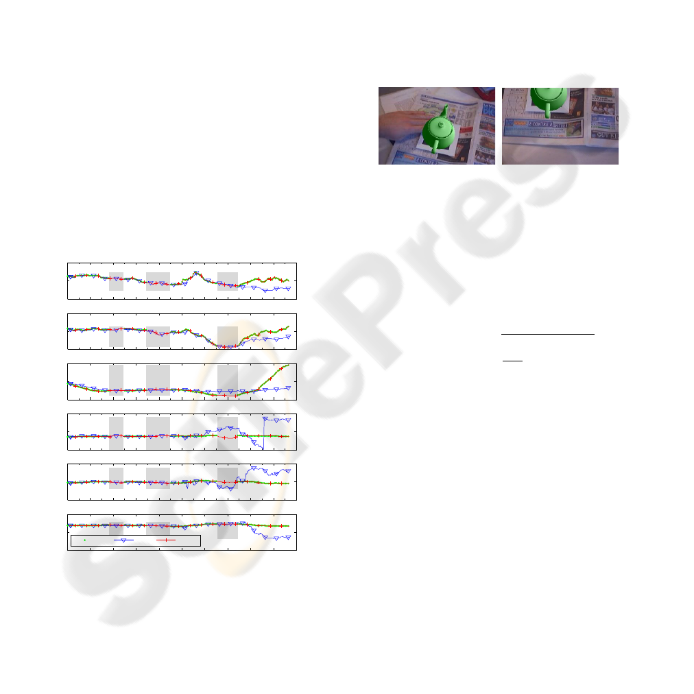
Figure 4 shows the estimation of the FPCT and our

approach (one realisation). Note that the rotation is

expressed in Euler angles converted from the rotation

quaternion. The estimate of the MCT (green dots)

−100

100

Trans X [mm]

−100

100

Trans Y [mm]

400

600

800

Trans Z [mm]

200

400

Rot X [º]

−100

100

Rot Y [º]

0 100 200 300 400 500 600 700 800 900 1000

−200

200

Rot Z [º]

Frame

MCT FPCT Fusion

Figure 4: First experiment. Translation and rotation in X,Y

and Z axes. Shaded regions represent occlusions (Manually

produced: frames 182-246, 345-448. Marker partially out

of FoV: frames 655-744).

is difﬁcult to observe because it is very close to the

ﬁltered estimate of our approach, except during the

occlusions, where no output is produced at all. The

FPCT (inverted triangles) is capable of tracking de-

spite the ﬁrst two occlusions. However, it looses track

after the third occlusion. This could be due to an in-

complete update step (only two 3D points are avail-

able while the marker is partially outside the FoV,

frames 655-744), leading to a bad prediction. As this

experiment illustrates, using the MC to update the

ﬁlter and the templates of the FPC produces better

results. In addition, using the FPC enables the fu-

sion to provide an estimate throughout the whole se-

quence. The fusion addresses the main drawbacks of

each component: partial occlusions for the MC, and

the viewpoint change for the FPC. Snapshots from

several frames of the augmented scene during occlu-

sions are shown in Figure 5.

(a) Occlusion (b) Escaping the FoV

Figure 5: First experiment. A virtual teapot placed on the

marker to show correct alignment.

In a second experiment, the adaptive ﬁltering pro-

posed is compared to similar work. Xu (Xu and Li,

2006) presented an adaptation method for 2DoF that

can be extended in terms of Eq. (10) to 6DoF as fol-

lows

ϕ = exp

−0.5

∑

[

(k) −

(k − 1)]

(k + 1) = max



min



1/ϕ;

i,max



;

i,min



, (11)

where

max

and

min

are the upper and lower bound

vectors and

is the nominal value for axis i. Note that

i,max

and

i,min

are ﬁxed ofﬂine to a single value

for the three rotation axes and another single value for

the three translation axes. Remark that the prediction

error in one axis affects all other hyper-parameters, as

ϕ is unique for all the axes. Consequently, the model

of process noise in one axis may grow even when

the real error in that axis is small. Moreover, the dy-

namic range of the variance of each axis is limited of-

ﬂine whereas our proposed dynamic tuning has only

a lower bound to insure stability when motion is al-

most static. In order to compare the proposed method

to this approximation of Xu’s approach, a second cus-

tom video sequence with several abrupt manoeuvres

is used. The upper bound is ﬁxed to the maximal

value achieved by our technique in this particular se-

quence. The lower bound is the same for both. The

variances in our method are initialised with the nomi-

nal values

. The variation bounds ∆

min

and ∆

max

are

VISAPP 2007 - International Conference on Computer Vision Theory and Applications

368

Table 2: Mean frame rates achieved for the MCT and FPCT

individually, and for our fusion ﬁlter updated from one or

the other cue.

Tracker

frame rate [Hz]

MCT 26.9

FPCT (1000 particles) 19.1

Fusion (update with MC) 23.8

Fusion (update with FPC) 17.9

5 CONCLUSION

We have presented a combination of video trackers

within a particle ﬁlter framework. The ﬁlter uses two

cues provided by a marker-based approach and a fea-

ture point-based one. The motion model is adapted

online according to the distance between past esti-

mates.

Experiments show that the proposed combination

produces a synergy. The system tolerates occlusions

and changes of illumination. Independent adaptive

tuning for the model of each DoF demonstrates su-

perior performance in front of manoeuvres.

In our future research, we will focus on extending

the FPC to feature points beyond the four corners of

the marker and enhancing their viewpoint sensibility.

ACKNOWLEDGEMENTS

The ﬁrst author is supported by the Swiss National

Science Foundation (grant number 200021-113827),

and by the European Networks of Excellence K-

SPACE and VISNET2.

REFERENCES

Allen, B., Bishop, G., and Welch, G. (2001). Tracking:

Beyond 15 minutes of thought. In SIGGRAPH.

Arulampalam, M., Maskell, S., Gordon, N., and Clapp,

T. (2002). A tutorial on particle ﬁlters for on-

line nonlinear/non-gaussian bayesian track ing. IEEE

Trans. on Signal Processing, 50(2):174–188.

Azuma, R. and Bishop, G. (1995). Improving static and

dynamic registration in an optical see-through HMD.

In SIGGRAPH, pages 197–204. ACM Press.

Chai, L., Nguyen, K., Hoff, B., and Vincent, T. (1999). An

adaptive estimator for registration in augmented real-

ity. In IWAR, pages 23–32.

Claus, D. and Fitzgibbon, A. (2004). Reliable ﬁducial de-

tection in natural scenes. In European Conference on

Computer Vision (ECCV), volume 3024, pages 469–

480. Springer-Verlag.

Davison, A. (2003). Real-time simultaneous localisation

and mapping with a single camera. In ICCV.

Fiala, M. (2005). ARTag, a ﬁducial marker system using

digital techniques. In CVPR, volume 2, pages 590–

596.

Ichimura, N. (2002). Stochastic ﬁltering for motion trajec-

tory in image sequences using a monte carlo ﬁlter with

estimation of hyper-parameters. In ICPR, volume 4,

pages 68–73.

Kanbara, M., Fujii, H., Takemura, H., and Yokoya, N.

(2000). A stereo vision-based augmented reality sys-

tem with an inertial sensor. In ISAR, pages 97–100.

Kato, H. and Billinghurst, M. (1999). Marker tracking and

HMD calibration for a video-based augmented reality

conferencing system. In IWAR, pages 85–94.

Koller, D., Klinker, G., Rose, E., Breen, D., Wihtaker,

R., and Tuceryan, M. (1997). Real-time vision-based

camera tracking for augmented reality applications. In

ACM Virtual Reality Software and Technology.

Maybeck, P. S. (1982). Stochastic Models, Estimation, and

Control, volume 141-2, chapter Parameter uncertain-

ties and adaptive estimation, pages 68–158. Academic

Press.

Najaﬁ, H., Navab, N., and Klinker, G. (2004). Automated

initialization for marker-less tracking: a sensor fusion

approach. In ISMAR, pages 79–88.

Okuma, T., Kurata, T., and Sakaue, K. (2003). Fiducial-

less 3-d object tracking in ar systems based on the in-

tegration of top-down and bottom-up approaches and

automatic database addition. In ISMAR, page 260.

Pupilli, M. and Calway, A. (2005). Real-time camera track-

ing using a particle ﬁlter. In British Machine Vision

Conference, pages 519–528. BMVA Press.

Satoh, K., Uchiyama, S., Yamamoto, H., and Tamura,

H. (2003). Robot vision-based registration utilizing

bird’s-eye view with user’s view. In ISMAR, pages

46–55.

Vacchetti, L., Lepetit, V., and Fua, P. (2004). Combining

edge and texture information for real-time accurate 3d

camera tracking. In ISMAR, Arlington, VA.

Xu, X. and Li, B. (2006). Rao-blackwellised particle ﬁl-

ter with adaptive system noise and its evaluation for

tracking in surveillance. In Visual Communications

and Image Processing (VCIP). SPIE.

You, S. and Neumann, U. (2001). Fusion of vision and gyro

tracking for robust augmented reality registration. In

IEEE Virtual Reality (VR), pages 71–78.

You, S., Neumann, U., and Azuma, R. (1999). Hybrid iner-

tial and vision tracking for augmented reality registra-

tion. In IEEE Virtual Reality (VR), pages 260–267.

Zhang, X., Fronz, S., and Navab, N. (2002). Visual marker

detection and decoding in AR systems: A comparative

study. In ISMAR, pages 97–106.

VISAPP 2007 - International Conference on Computer Vision Theory and Applications

370