
GAP FILLING IN 3D VESSEL LIKE PATTERNS WITH TENSOR
FIELDS
Application to High Resolution Computed Tomography Images of Vessel Networks
Laurent Risser, Franck Plourabou
´
e
IMFT, Universit
´
e Paul Sabatier, av. du Pr. Camille Soula, 31400 Toulouse, France
Xavier Descombes
INRIA, 2004 route des Lucioles, BP93, 06902, Sophia Antipolis Cedex, France
Keywords:
Network, vessel extraction, skeleton, tensor voting, gap filling.
Abstract:
We present an algorithm for merging discontinuities in three-dimensional (3D) images of tubular structures.
The application of the proposed method is associated with large 3D images presenting undesirable discontinu-
ities. In order to recover the real network topology, we need to fill the gap between the closest discontinuous
tubular segments. We present a new algorithm to achieve this goal based on a tensor voting method. This
algorithm is robust, relatively fast and does not require numerous parameters nor manual intervention. Repre-
sentative results are illustrated on real 3D micro-vascular networks.
1 INTRODUCTION
The extraction of vascular networks is an important
problem in numerous medically oriented image anal-
ysis tasks. In this context many methods for extract-
ing vessel networks from noisy images have been de-
veloped (Lorigo et al., 2001; Krissian et al., 2000;
Zana and Klein, 2001; McInerney and Terzopoulos,
1996). One important issue concerning these extrac-
tion techniques is that they may cause the boundaries
of a structure to be indistinct and disconnected. In
an attempt to solve the problem some authors have
proposed specific methods associated with the need
for topological preservation in the extraction of vas-
cular networks (Quek and Kirbas, 2001). Neverthe-
less, despite the large number of vessel segmentation
methods put forward, the issue of gap filling has not
been addressed much in the context of 3-D medical
imaging. To the best of our knowledge only one gap
filling algorithm for vascular networks has been de-
veloped (Szymczak et al., 2005). Discontinuities in
the network limit the topological analysis, a drawback
which is becoming important in an increasing number
of medical applications (Bullitt and Aylward, 2005).
There is indeed a growing demand for better analysis
of micro-vascular structures (Popel et al., 1999). Im-
proving vessel connectivity in those networks is thus
a key issue, and it is the goal of the present paper.
2 PRIOR WORK ON GAP
FILLING IN TUBULAR
STRUCTURES
In order to generalize the context of 3D vascular net-
works, we will consider it as a network of tubular
structures. In the following, the term segment refers
to a part of this network. A segment may be defined
between two bifurcations, between one bifurcation
and one extremity of the tubular structure or between
two extremities of the tubular structure (fig.2).
Although the problem of gap filling in tubular
structures has not been widely addressed in 3D, it has
been the object of much attention in 2D. For example,
in the field of remote sensing, the extraction of road
networks requires gap filling. Blockages, crossroads,
shadows and variations of the background or road in-
tensity may cause gaps in the road network. In this
context an algorithm of road extraction improvement
by using higher-order active contours is proposed in
(Rochery et al., 2004). In (Tesser and Pavlidis, 2000),
road network mid-lines are first extracted. The mid-
line endpoints are thus easily detected. They become
the seeds of the gap filling algorithm. In (Lacoste
et al., 2005), a global optimization solution with sim-
ulated annealing for gap filling in line networks is ap-
plied. The cost function depends on the configuration
46
Risser L., Plouraboué F. and Descombes X. (2007).
GAP FILLING IN 3D VESSEL LIKE PATTERNS WITH TENSOR FIELDS - Application to High Resolution Computed Tomography Images of Vessel
Networks.
In Proceedings of the Second International Conference on Computer Vision Theory and Applications - IFP/IA, pages 46-52
Copyright
c
SciTePress
of the overall line endpoint pairs.
Perceptual organization techniques (Marr, 1982)
are especially interesting for the problem of gap fill-
ing in vessel like patterns. Those techniques aim at
grouping the primitives contained in a data set into
perceptual structures. Those primitives are usually
called tokens. For example, in (Parent and Zucker,
1989) a reliability measure on whether two isolated
segment ends seem to be on the same arc of a cir-
cle is given. Experiments have been carried out on
biomedical images in order to merge vessel pieces.
In (Saund, 1992) gaps between tokens are filled with
a fine to coarse process. In (Heitger and Von der
Heydt, 1993), several features are distinguished in
shape boundaries. They are thus merged locally with-
out feedback. A rich expansion of perceptual organi-
zation techniques is tensor voting (Guy and Medioni,
1997). This technique was initially developed in order
to reconstruct shapes from point clouds. It allows the
simultaneous communication among various types of
tokens. Moreover the information exchange between
tokens uses tensor fields rather than scalar ones as
in other methods. The communication is thus much
richer. The initial algorithm has numerous evolutions
and adaptations. For example a multi-scale algorithm
for boundary inference is presented in (Tong et al.,
2004). In (Massad et al., 2002) a tensor field is built
using Gabor filters on a gray level image. The tensor
field is thus used to fill gaps between segments. In (Jia
and Tang, 2003), tensor voting is applied to curve end-
points in order to extrapolate and merge them. There-
fore, tensor voting provides an interesting formalism
for gap closure procedures in vessel networks.
3 MEHOD
3.1 Method Overview
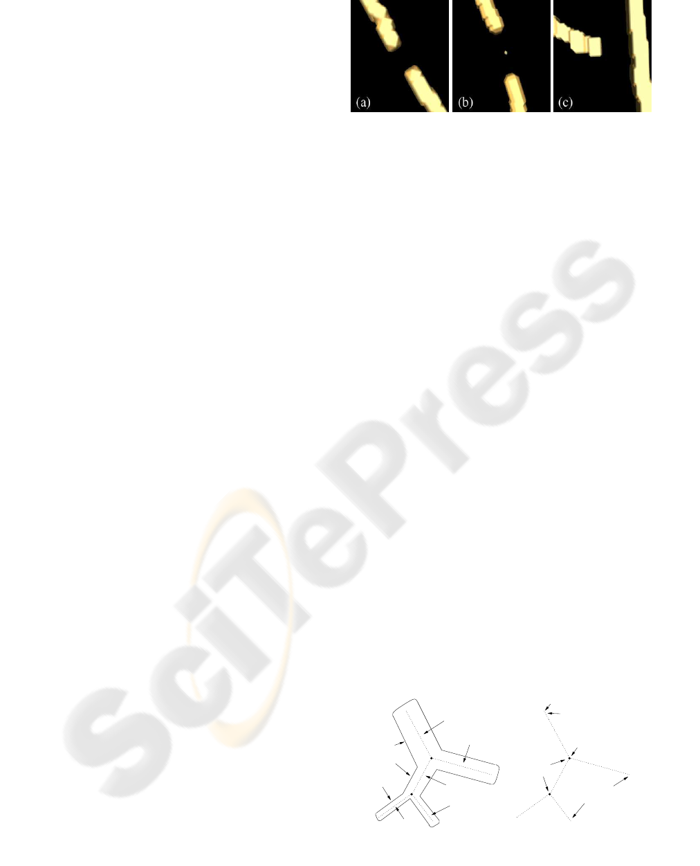
In the present paper, we distinguish three typical
cases of discontinuities: (1) A vessel is simply
disconnected (fig.1 (a)); (2) A vessel is disconnected.
The vessel is however detected at several voxels
within the gap (fig.1 (b)); (3) A vessel is discon-
nected just close to a bifurcation (fig.1 (c)). Most
of the current methods presented in section 2 which
could be applicable to 3D vascular network images
could only fill the first type of discontinuities. Our
method permits to treat efficiently the three cases of
discontinuities defined.
The initial data are the vascular network skeleton.
The following notations will be taken: a skeleton
point is an element. Each element contains the
Figure 1: (a) A simple gap. (b) Information remaining
within a gap. (c) Information lacks just after a bifurcation.
coordinates and the radius of the local section of the
shape. For each segment the elements are ordered as
a chain. Each chain is a S-segment (fig.2).
Two fields are required for the gap filling algo-
rithm: a tensor field T and a scalar field A. Each ten-
sor is represented by a 3×3 matrix. Each field can be
seen as a 3-D image of tensors for T and of scalars for
A. Both T and A size is [I,J,K]. This size has to be
large enough to contain the whole network. Indeed,
in order to describe the disconnected network, three
kinds of tokens will be extracted from the skeleton.
Those token will express themselves in T and A.
3.2 Tokens Description
Let α be the threshold number of elements which dif-
ferentiates a usual segment from an island. An island
is a segment which is so small that its directional as-
pect is not significant. We take α = 5. In order to de-
fine the tokens, we will distinguish three kinds of seg-
ments: 0-segments are not connected to any other seg-
ment. 1-segments have just one end connected to an
other segment. 2-segments have their two ends con-
nected. The tokens are then defined as follows (fig.3):
• Segment-end token: A non connected segment
end. The segment size is larger than α. A site
and a direction certainty are associated with each
segment end token.
• Island token: A 0-segment whose size is smaller
S−segment 1
S−segment 2
S−segment 3
S−segment 4
Isolated
endpoints
Element 1 (S−segment 1)
Element 2 (S−segment 1)
Node
S−segment 5
Segment 1
Segment 3
Segment 5
segment
endpoints
1
Element I (S−segment 1)
Figure 2: Notations used for the skeleton description. Ele-
ment I
1
designates the last element in the S-segment 1.
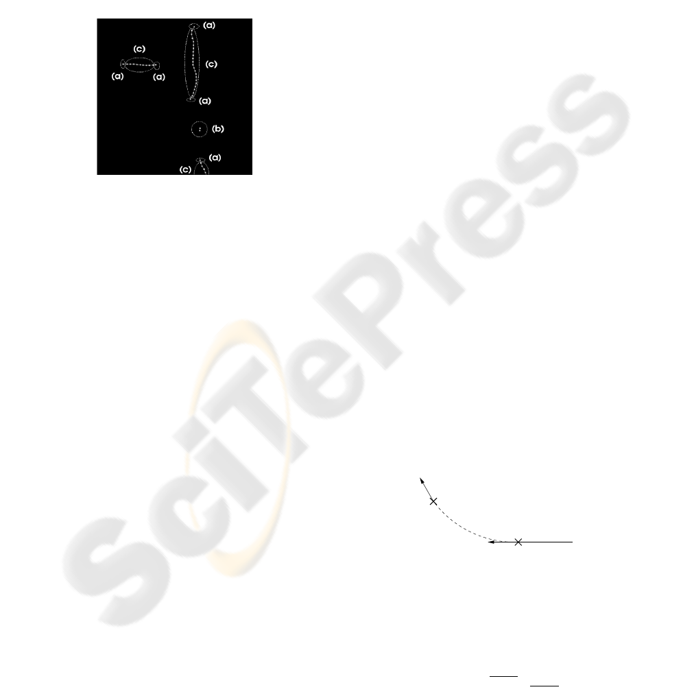
or equal to α. A site is associated with each island
token.
• Segment token: A 0-segment of size larger than
α or a 1-segment or a 2-segment. The elements
close to the ends are not taken into account be-
cause they correspond to segment end tokens.
Each element of the segment token is associated
with a site, a radius and a direction uncertainty
around the segment tangent. The radius expresses
the volume of each element.
Figure 3: The three types of tokens: (a) Segment-end to-
kens; (b) Island Token; (c) Segment tokens.
3.3 Scalar Field Construction
The tokens express their coordinates in the scalar field
A. Each class of token expresses itself in its own par-
ticular way.
An identifier is associated with the end of each S-
segment. This identifier is written in A at the coordi-
nates corresponding to the segment end. The coordi-
nates of A are integers whereas those of the segment
ends are floats. The exact coordinates are thus ap-
proximated in A. If two or more segment ends express
their coordinates in the same pixel of A the segment
ends are supposed to make up a node of the network.
This pixel is then set to zero. If one and only one
voxel express himself at a pixel of A the identifier is
kept and the segment end is a segment-end token.
As for the segment-ends, each island has an iden-
tifier. This identifier is written in A at the coordinates
of the island’s center. An island token is thus consid-
ered for each island.
The segments are also expressed in A using iden-
tifiers. Each element of the corresponding S-segment
puts the segment identifier in a sphere. This sphere is
centered in the element coordinates and its radius is
the embedded element’s radius. If the element sam-
pling is not dense enough to form an unbroken curve
in A, the points are interpolated.
3.4 Tensor Field Construction
The tokens as a whole express their direction certainty
in T (fig.5 (d)). Let us break T into several tensor
fields each expressing a token directional aspect. Let
TE
n
, n ∈ [1,N] be the tensor field created by the n
th
segment-end token, TI
m
, m ∈ [1,M] the tensor field
created by the m
th
island token and TS
q
, q ∈ [1,Q] the
tensor field created by the q
th
segment token. Thus,
for each point [i, j,k] of T :
T(i, j,k) =
N
∑
n=1
TE
n
(i, j,k)
+
M
∑
m=1
TI
m
(i, j,k) +
Q
∑
q=1
TS
q
(i, j,k)
(1)
This formula represents the communication be-
tween tokens. The construction and expression of
each token is slightly different than those proposed
in (Tong et al., 2004) or (Guy and Medioni, 1997).
In those papers, the tensor fields express a direction
uncertainty but, due to the expression we use for the
tokens, a direction certainty is more natural. Our ten-
sor fields thus embed a direction certainty. Let us now
describe the construction of each tensor field.
3.4.1 Segment-End Token
We assume a point P close to the segment end O. The
tangent to the segment in O is V. First, V and OP are
chosen as normalized unit vectors (||V|| = ||OP|| =
1). Let W be such that:
W = 2OP(OP.V) − V (2)
The vector W is the oriented tangent at P to
the circle Ci which contains O and P and which is
tangent at O to V.
V
O
P
W
Figure 4: Arc of circle used for the construction of the ten-
sor field which express a segment-end token direction cer-
tainty.
The vector W is weighted as follows:
w
∗
= e
−
r
2
+cϕ
2
σ
2
W
||W||
(3)
Where r is the length of the arc
c
OP of the circle
Ci and ϕ its curvature. The coefficient σ is the scale
of the analysis and c the influence ratio between the
proximity and the curvature. The tensor TE is then
defined from w
∗
as TE = w
∗
⊗ w
∗
, where ⊗ is the
tensor product. At P, the tensor TE then corresponds
to the vote of the segment end token located at O (fig.5
(a)).
3.4.2 Island Token
Let C be the center point of the segment representing
an island token and P a point close to C. The vector
CP is then weighted as for the segment-end token ex-
cept that the length of the arc of the circle is replaced
by the distance between C and P and that the curva-
ture is no longer used :
cp
∗
= e
−
||CP||
2
σ
2
CP
||CP||
(4)
The tensor TI is then defined from vector cp
∗
:
TI = cp
∗
⊗ cp
∗
. At P, the tensor TI corresponds to
the vote of the island token located at C (fig.5 (b)).
3.4.3 Segment Token
In order to build the tensor voting field of a segment
token we first create a vector field. Let V(P) be the
vector of the field at the point P. This vector aims at
the nearest element of the segment token N. Its norm
is ||NP|| − Rad(P) where Rad(P) is the radius of the
skeleton at the element expressed in P. If ||NP|| >
Rad(P) the norm is null. The segment token is thus
weighted:
np
∗
= e
−
(||V(P)||−A(P))
2
σ
2
V(P)
||V(P)||
(5)
The tensor TS is then defined from vector np
∗
: TS =
np
∗
⊗ np
∗
. At P, the tensor TS corresponds to the
vote of the segment token at the nearest point to N of
its skeleton (fig.5 (c)).
3.5 Tokens Junction
As already proposed in (Tong et al., 2004) or (Guy
and Medioni, 1997) we compute the saliency map S
to a curve by using the tensor voting field T (fig.6).
Each point of this map contains a scalar value which
measures the saliency of the tensor voting field to a
curve. Let λ
1
(i, j,k), λ
2
(i, j,k) and λ
3
(i, j,k) be the
eigenvalues of the tensor T(i, j,k) with |λ
1
(i, j,k)| >
|λ
2
(i, j,k)| > |λ
3
(i, j,k)|. Since our choice on the ten-
sor construction differs from those of (Tong et al.,
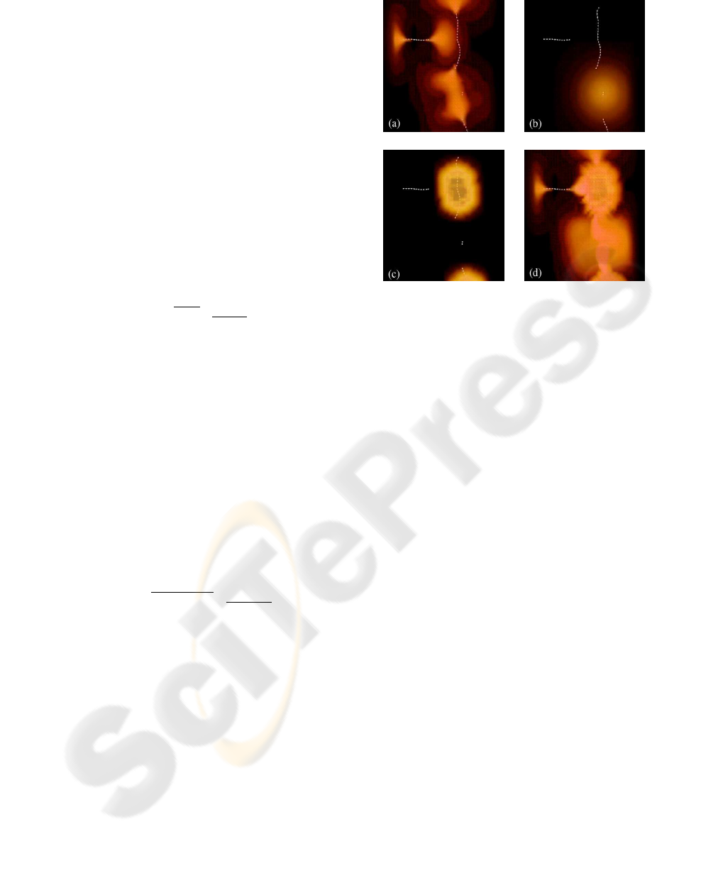
Figure 5: Expression of the direction certainty energy E of
the tokens with E = (
∑
3
i=1
∑
3
j=1
T
2
i, j
)
1/2
. (a) Segment-end
token energy E(TP). (b) Island token energy E(TI). (c)
Segment token energy E(TS). (d) Total energy E(T).
2004; Guy and Medioni, 1997) we self-consistently
define the saliency to a curve at the point [i, j, k] as
S(i, j,k) = λ
1
(i, j,k) −λ
2
(i, j,k) (6)
The tokens are merged with paths following iter-
atively the watersheds of the saliency map S. Each
segment end token is the seed of a path. Let P
i
be a
point of the path and D
i
the direction associated to P
i
.
The point P
i+1
is estimated as follow:
P
i+1
= argmax S(p)
p ∈ N
3×3×3
(P
i
)
pP
i
.D
i
> 0
(7)
The direction D
i+1
is thus: D
i+1
= P
i+1
P
i
. The
path is stopped according to four criteria: (1) The
path leads to another segment end token. The two
segments are then joined by the path (fig.6 (a)). (2)
The path conducts to a segment token. The segment
is divided at the nearest element token to the junction
point. The segment end token join the segment token
at this point (fig.6 (b)). (3) The path leads to an is-
land token. The segment end token is then joined to
the island token by the path (fig.6 (c)). The island to-
ken and its contribution in the tensor voting field are
deleted. The expression of the newly created segment
end token is added to the tensor voting field. An other
watersheds path starts thus from the end of the new
segment in order to try another junction (fig.6 (d)).
(4) The path is stopped if the value of the saliency
map is lower than a given threshold or if it reaches
the boundary of the image.
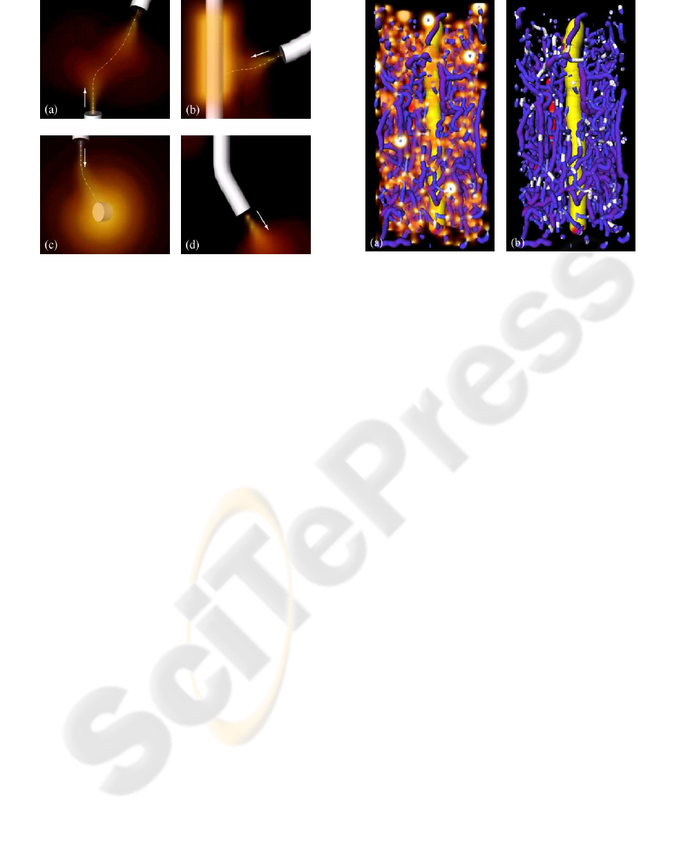
Figure 6: Different cases of path. The voltex represents the
saliency map. (a) Segment end token to segment end token.
(b) Segment end token to segment token. (c) Segment end
token to island token (part 1). (d) Segment end token to
island token (part 2).
The radii of the segments created depends on the
radii in the segment-end token. They are linearly
interpolated if the junction is drawn between two
segment-end tokens and are equal to the radius at the
segment-end in the two other cases. At each itera-
tion, the junction test between the path and a token
is computed by using the scalar field. When a path
joins a token identifier, the token is thus immediately
recognized. The token junction algorithm avoid thus
the comparison of token pairs. The whole algorithm
is then of order O(E) with E the number of segment
end tokens. It is thus especially adapted to large net-
works.
4 APPLICATION
The gap filling treatment was tested both on real intra-
cortical micro-vascular networks (fig.7) and on phan-
tom networks (fig. 8 and 9). The images of real net-
work were obtained using synchrotron tomography
imaging at the European Synchrotron Radiation Fa-
cility (Plourabou
´
e et al., 2004). They contain from
5000 to 50000 segments. The resolution is about one
micron, so that one can obtain a 3D image of the en-
tire vascular network on volumes as large as 8mm
3
.
The image contrast between the vessels and the sur-
rounding tissues is very good. The image binarization
with hysteresis thresholding followed by skeletoniza-
tion leads thus to a very satisfactory result. However,
the observed vascular network contains some discon-
Figure 7: Treatment of the sample of a real network. The
sample contains 822 segments. Calculations require 499
seconds and 689 Mo. (a) Skeleton and saliency map. The
voltex represents the saliency map. (b) Filled skeleton.
Filled gaps are in white.
tinuities. The gap filling algorithm is then applied to
those networks. The evaluation of the algorithm effi-
ciency is tough on a real 3D network mainly because
the rigorous estimation of the number of gaps to fill is
complicated. The thorough visualization of the gaps
filled requires also a large amount of time because of
the 3D. The gap filling algorithm is therefore roughly
estimated visually (fig.7). The results look perceptu-
ally good. Almost all the gaps seem filled when the
scale and curvature parameters are adapted to the net-
work. All calculations were carried out on a Linux
PC with an intel Xeon 2,13 GHz processor and 4 Go
of RAM. The comments of the figure 7 give an idea
of the time and the memory required.
In order to measure quantitatively the gap filling
algorithm, clean 2D phantom networks were created.
They were extracted from real intra-cortical networks.
These samples were thin and especially clean. They
were then projected onto a plan. The crossings be-
tween segments due to the projection were erased.
Then the networks were repaired so that our gap fill-
ing algorithm did not improve them any more. Those
networks became the reference networks. Damaged
networks were obtained using the reference networks.
Their deterioration was controlled. It was then possi-
ble to measure the efficiency of the damaged network
reconstruction. The deterioration is processed in the
following way. A given proportion of points of the
network were the centers of gaps. The size of each
of these gaps followed a Gaussian law. Once the net-
work had been disconnected, noise was added to the
background. A given density of island tokens was ho-
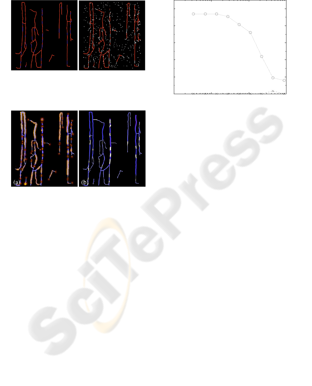
Figure 8: (left) A reference network. The parts removed
from the network are blue. (right) A reconstructed damaged
network with 198.10
−6
islands per voxel (A thickness of 20
voxels is considered).
Figure 9: Treatment of a phantom network. The network
contains 71 segments. Calculations require 42 seconds and
71 Mo.(a) Skeleton and saliency map. The voltex represents
the saliency map. (b) Filled skeleton. Filled gaps are in
white.
mogeneously distributed around the disconnected net-
work. Figures 8 and 9 illustrate the deterioration and
reconstruction of a reference network.
The influence of noise on our gap filling al-
gorithm will now be evaluated. Several densities
of noise island tokens and a given number of dis-
continuities were injected into the networks. The
noised networks were then treated with the gap
filling method. Figure 10 represents the algorithm
efficiency in function of the noise injected. Both
the proportion of gaps filled and the number of
fake junctions in the expected number of junctions
versus noise was then evaluated. Fake junctions
are due to two segment-end tokens which join the
same noise island. They are uncommon and only
found on very noisy networks. The number of good
junctions was high and stable for moderately noised
networks. For highly noised networks, the number
of good gaps filled decreases almost linearly in the
semi-logarithmic representations of figures indicating
a sensible influence of the noise ratio. At this stage,
10
−6
10
−5
10
−4
10
−3
Noise (number of islands injected / voxel)
0
20
40
60
80
100
Gaps Filled (percents)
Figure 10: Gap filling efficiency compared to the noise. Cir-
cles: Proportion of good gap closures. Crosses: Number of
false gap closures on the expected number of gap closures.
the gaps that cannot be filled anymore are mainly
associated with segment-end tokens which are useful
for the network reconstruction and which now join a
noisy island.
5 CONCLUSION
We have proposed a new method for fast and robust
gap filling in large 3D tubular structurs networks. The
three typical cases of discontinuities highlighted in
the introduction are easily taken into account. The
network is improved by the junction of tokens that
would perceptually be attributed to the same vessel.
The results look perceptually natural. The gap filling
procedure does not require numerous parameters nor
manual interventions. The whole algorithm is of or-
der O(E) with E the number of segment end tokens. It
is thus especially adapted to large networks. The use
of a tensor field requires however a large amount of
memory. Nevertheless, the required memory can be
minimized by the use of a sliding window inside the
image. The proposed method shall prove very useful
in the topology reconstruction of micro-vascular net-
works. It is interesting to note that this method can be
used for post-treating medical images as for example
in angiography or scanners. The formalism can also
be easily generalized to any other dimension, includ-
ing 2D, with a large number of applications.

ACKNOWLEDGEMENTS
The research was supported by ASUPS A03 and
ASUPS A05 of Paul Sabatier University, Toulouse,
France; the French Ministry of Research; the Eu-
ropean Synchrotron Research Facilities (MD99 and
MD26); and the French Foundation for Medical Re-
search (Fondation pour la Recherche M
´
edicale). The
authors thank Vincent Gratsac for technical support.
REFERENCES
Bullitt, E. and Aylward, S. (2005). Three-dimensional blood
vessel trees: Clinical needs and applications. RSNA
Syllabus on Diagnostic Imaging Physics.
Guy, G. and Medioni, G. (1997). Inference of surfaces,
3d curves, and junctions from sparse, noisy, 3d data.
IEEE PAMI, 26(11):1265–1277.
Heitger, F. and Von der Heydt, R. (1993). A computational
model of neural contour processing: Figure-ground
segregation and illusory contours. In Proc. Int’l Conf.
Computer Vision, pages 32–40.
Jia, J. and Tang, C.-K. (2003). Image repairing: Robust
image synthesis by adaptative Nd tensor voting. In
Proceedings IEEE CVPR.
Krissian, K., Malandain, G., and Ayache, N. (2000). Model-
based detection of tubular structures in 3d images.
Computer Vision and Image Understanding, 80:130–
171.
Lacoste, C., Descombes, X., and Zerubia, J. (2005). Point
processes for unsupervised line network extraction in
remote sensing. IEEE PAMI, 27(10):1568–1579.
Lorigo, L., Faugeras, O., Grimson, W., Keriven, R., Kiki-
nis, R., Nabavi, A., and Westin, C.-F. (2001). Curves:
Curve for vessel segmentation. Medical Image Anal-
ysis, 5:195–206.
Marr, D. (1982). Vision. W.H. Freeman and Company.
Massad, A., Bab
´
os, M., and Mertsching, B. (2002). Percep-
tual grouping in grey-level images by combination of
gabor filtering and tensor voting. In ICPR02.
McInerney, T. and Terzopoulos, D. (1996). Defomable
models in medical image analysis: a survey. Medical
Image Analysis, 1(2):91–108.
Parent, P. and Zucker, S. (1989). Trace inference, curva-
ture consistency, and curve detection. IEEE PAMI,
11(8):823–839.
Plourabou
´
e, F., Cloetens, P., Fonta, C., Steyer, A., Lauw-
ers, F., and Marc-Vergnes, J. (2004). High resolution
x-ray imaging of vascular networks. J. Microscopy,
215(2):139–148.
Popel, A., Pries, A., and Slaaf, D. (1999). Developments
in the microcirculation physiome project. Journal of
Vascular Biology, 36:253–255.
Quek, F. and Kirbas, C. (2001). Vessel extraction in medi-
cal images by wave-propagation and traceback. IEEE
Transactions on Medical Imaging, 20(2):117–131.
Rochery, M., Jermyn, I., and Zerubia, J. (2004). Gap closure
in (road) networks using higher-order active contours.
In Proc. IEEE ICIP 2004.
Saund, E. (1992). Labelling of curvilinear structure across
scales by token grouping. In Proc. CVPR, pages 257–
263.
Szymczak, A., Tannenbaum, A., and Mischaikow, K.
(2005). Coronary vessel cores from 3d imagery: a
topological approach. In Proceedings of SPIE - Med-
ical Imaging 2005: Image Processing, volume 5747,
pages 505–513.
Tesser, H. and Pavlidis, T. (2000). Roadfinder front end:
An automated road extraction system. In Proc. ICPR,
pages 338–341.
Tong, W., Tang, C., Mordohai, P., and Medioni, G. (2004).
First order augmentation to tensor voting for boundary
inference and multiscale analysis in 3d. IEEE trans-
actions on pattern analysis and machine intelligence,
26(5):594–611.
Zana, Z. and Klein, J. (2001). Segmentation of vessel-like
patterns using mathematical morphology and curva-
ture evaluation. IEEE Transactions on Image Process-
ing, 10(7):1010–1019.
