COMPACT (AND ACCURATE) EARLY VISION PROCESSING IN

THE HARMONIC SPACE

Silvio P. Sabatini, Giulia Gastaldi, Fabio Solari

Dipartimento di Ingegneria Bioﬁsica ed Elettronica, University of Genoa, via Opera Pia 11a, Genova, Italy

Karl Pauwels, Marc van Hulle

Laboratorium voor Neuro- en Psychofysiologie, K.U.Leuven, Belgium

Javier D

ıaz, Eduardo Ros

Departamento de Arquitectura y Tecnologia de Computadores, University of Granada, Spain

Nicolas Pugeault

School of Informatics, University of Edinburgh, U.K.

Norbert Kr

uger

The Maersk Mc-Kinney Moller Institute, University of Southern Denmark, Odense, Denmark

Keywords:

Phase-based techniques, multidimensional signal processing, ﬁlter design, optic ﬂow, stereo vision.

Abstract:

The efﬁcacy of anisotropic versus isotropic ﬁltering is analyzed with respect to general phase-based metrics for

early vision attributes. We veriﬁed that the spectral information content gathered through oriented frequency

channels is characterized by high compactness and ﬂexibility, since a wide range of visual attributes emerge

from different hierarchical combinations of the same channels. We observed that it is preferable to construct

a multichannel, multiorientation representation, rather than using a more compact representation based on an

isotropic generalization of the analytic signal. The complete harmonic content is then combined in the phase-

orientation space at the ﬁnal stage, only, to come up with the ultimate perceptual decisions, thus avoiding

an “early condensation” of basic features. The resulting algorithmic solutions reach high performance in

real-world situations at an affordable computational cost.

1 INTRODUCTION

Although the basic ideas underlying early vision

appear deceptively simple and their computational

paradigms are known for a long time, early vision

problems are difﬁcult to quantify and solve. More-

over, in order to have high algorithmic performance

in real-world situations, a large number of channels

should be integrated with high efﬁciency. From a

computational point of view, the visual signal should

be processed in a “unifying” perspective that will al-

low us to share the maximum number of resources.

From an implementation point of view, the resulting

algorithms and architectures could fall short of their

expectations when the high demand of computational

resources for multichannel spatio-temporal ﬁltering

of high resolution images conﬂicts with real-time re-

quirements. Several approaches and solutions have

been proposed in the literature to accelerate the com-

putation by means of dedicated hardware (e.g., see

(Diaz et al., 2006; Kehtarnavaz and Gamadia, 2005)).

Yet, the large number of products that must be com-

puted to calculate each single pixel of each single

frame for a couple of stereo images and at each time

step still represents the main bottleneck. This is par-

ticularly true for stereo and motion problems to con-

213

P. Sabatini S., Gastaldi G., Solari F., Pauwels K., van Hulle M., Díaz J., Ros E., Pugeault N. and Krüger N. (2007).

COMPACT (AND ACCURATE) EARLY VISION PROCESSING IN THE HARMONIC SPACE.

In Proceedings of the Second International Conference on Computer Vision Theory and Applications - IFP/IA, pages 213-220

 SciTePress

struct 3D representations of the world, for which es-

tablishing image correspondences in space and space-

time is a prerequisite, but also their most challenging

part.

In this paper, we propose (1) to deﬁne a systematic

approach to obtain a “complete” harmonic analysis of

the visual signal and (2) to integrate efﬁcient multi-

channel algorithmic solutions to obtain high perfor-

mance in real-world situations, and, at the same time,

an affordable computational load.

2 MULTICHANNEL BANDBASS

REPRESENTATION

An efﬁcient (internal) representation is necessary to

guarantee all potential visual information can be made

available for higher level analysis. At an early level,

feature detection occurs through initial local quanti-

tative measurements of basic image properties (e.g.,

edge, bar, orientation, movement, binocular disparity,

colour) referable to spatial differential structure of the

image luminance and its temporal evolution (cf. lin-

ear cortical cell responses). Later stages in vision can

make use of these initial measurements by combin-

ing them in various ways, to come up with categor-

ical qualitative descriptors, in which information is

used in a non-local way to formulate more global spa-

tial and temporal predictions. The receptive ﬁelds of

the cells in the primary visual cortex have been in-

terpreted as fuzzy differential operators (or local jets

(Koenderink and van Doorn, 1987)) that provide reg-

ularized partial derivatives of the image luminance in

the neighborhood of a given point x = (x, y), along

different directions and at several levels of resolution,

simultaneously. Given the 2D nature of the visual sig-

nal, the spatial direction of the derivative (i.e., the ori-

entation of the corresponding local ﬁlter) is an impor-

tant “parameter”. Within a local jet, the directionally

biased receptive ﬁelds are represented by a set of sim-

ilar ﬁlter proﬁles that merely differ in orientation.

Alternatively, considering the space/spatial-

frequency duality (Daugman, 1985), the local jets

can be described through a set of independent spatial-

frequency channels, which are selectively sensitive

to a different limited range of spatial frequencies.

These spatial-frequency channels are equally apt as

the spatial ones. From this perspective, it is formally

possible to derive, on a local basis, a complete

harmonic representation (phase, energy/amplitude,

and orientation) of any visual stimulus, by deﬁning

the associated analytic signal in a combined space-

frequency domain through ﬁltering operations with

complex-valued band-pass kernels. Formally, due to

the impossibility of a direct deﬁnition of the analytic

signal in two dimensions, a 2D spatial frequency

ﬁltering would require an association between spatial

frequency and orientation channels. Basically, this

association can be handled either (1) ‘separately’,

for each orientation channel, by using Hilbert pairs

of band-pass ﬁlters that display symmetry and

antisymmetry about a steerable axis of orientation,

or (2) ‘as-a-whole’, by introducing a 2D isotropic

generalization of the analytic signal: the monogenic

signal (Felsberg and Sommer, 2001), which allows us

to build isotropic harmonic representations that are

independent of the orientation (i.e., omnidirectional).

By deﬁnition, the monogenic signal is a 3D phasor

in spherical coordinates and provides a framework

to obtain the harmonic representation of a signal

respect to the dominant orientation of the image that

becomes part of the representation itself.

In the ﬁrst case, for each orientation channel θ, an

image I(x) is ﬁltered with a complex-valued ﬁlter:

(x) = f

(x) − if

(x) (1)

where f

(x) is the Hilbert transform of f

(x) with re-

spect to the axis orthogonal to the ﬁlter’s orientation.

This results in a complex-valued analytic image:

(x) = I ∗ f

(x) = C

(x) + iS

(x) , (2)

where C

(x) and S

(x) denote the responses of the

quadrature ﬁlter pair. For each spatial location,

the amplitude ρ

+ S

and the phase φ

arctan(S

) envelopes measure the harmonic infor-

mation content in a limited range of frequencies and

orientations to which the channel is tuned.

In the second case, the image I(x) is ﬁltered with

a spherical quadrature ﬁlter (SQF):

(x) = f(x) −(i, j) · f

(x) (3)

deﬁned by a rotation invariant even f(x) ﬁlter)

and a vector-valued isotropic odd ﬁlter f

(x) =

( f

R ,1

(x), f

R ,2

(x))

, obtained by the Riesz transform

of f(x) (Felsberg and Sommer, 2001). This results in

a monogenic image:

(x) = I ∗ f

(x) = C(x) + (i, j)S(x) (4)

= C(x) + iS

(x) + jS

(x)

where, using the standard spherical coordinates,

C(x) = ρ(x)cosϕ(x)

(x) = ρ(x)sinϕ(x) cosϑ(x)

(x) = ρ(x)sinϕ(x) sinϑ(x) .

The amplitude of the monogenic signal is the vec-

tor norm of f

: ρ =

+ S

, as in the case

of the analytic signal, and, for an intrinsically one-

dimensional signal, ϕ and ϑ are the dominant phase

and the dominant orientation, respectively.

In this work, we want to analyze the efﬁcacy of

the two approaches in obtaining a complete and ef-

ﬁcient representation of the visual signal. To this

end, we consider, respectively, a discrete set of ori-

ented (i.e., anisotropic) Gabor ﬁlters and a triplet of

isotropic spherical quadrature ﬁlters deﬁned on the

basis of the monogenic signal. Moreover, as a choice

in the middle between the two approaches, we will

also take into consideration the classical steerable ﬁl-

ter approach (Freeman and Adelson, 1991) that allows

a continuous steerability of the ﬁlter respect to any

orientation. In this case, the number of basis kernels

to compute the oriented outputs of the ﬁlters depends

on the derivative order (n) of a Gaussian function. The

basis ﬁlters corresponding to n = 2 or n = 4 turned out

as an acceptable compromise between the representa-

tion efﬁcacy and the computational efﬁciency.

For all the ﬁlters considered, we chose the de-

sign parameters to have a good coverage of the space-

frequency domain and to keep the spatial support (i.e.,

the number of taps) to a minimum, in order to cut

down the computational cost. Therefore, we deter-

mined the smallest ﬁlter on the basis of the highest al-

lowable frequency without aliasing, and we adopted

a pyramidal technique (Adelson et al., 1984) as an

economic and efﬁcient way to achieve a multireso-

lution analysis (see also Section 3.2). Accordingly,

we ﬁxed the maximum radial peak frequency (ω

)

by considering the Nyquist condition and a constant

relative bandwidth of one octave (β = 1), that al-

lows us to cover the frequency domain without loss

of information. For Gabor and steerable ﬁlters, we

should also consider the minimum number of ori-

ented ﬁlters to guarantee a uniform orientation cov-

erage. This number still depends on the ﬁlter band-

width and it is related to the desired orientation sen-

sitivity of the ﬁlter (e.g., see (Daugman, 1985; Fleet

and Jepson, 1990)); we veriﬁed that, under our as-

sumptions, it is necessary to use at least eight orien-

tations. To satisfy the quadrature requirement all the

even symmetric ﬁlters have been “corrected” to can-

cel the DC sensitivity. The monogenic signal has been

constructed from a radial bandpass ﬁlter obtained by

summing the corrected bank of oriented even Gabor

ﬁlters. All the ﬁlters have been normalized prior to

their use in order to have constant unitary energy. A

detailed description of the ﬁlters used can be found at

www.pspc.dibe.unige.it/VISAPP07/

3 PHASE-BASED EARLY VISION

ATTRIBUTES

3.1 Basic Principles

During the last decades, the phase from local band-

pass ﬁltering has gained increasing interest in the

computer vision community and has led to the de-

velopment of a wide number of phase-based feature

detection algorithms in different application domains

(Sanger, 1988; Fleet et al., 1991; Fleet and Jepson,

1990; Fleet and Jepson, 1993; Kovesi, 1999; Gau-

tama and Van Hulle, 2002). Yet, to the best of our

knowledge, a systematic analysis of the basic descrip-

tive properties of the phase has never been done. One

of the key contributions of this paper is the formu-

lation a single uniﬁed representation framework for

early vision grounded on a proper phase-based met-

rics. We veriﬁed that the resulting representation

is characterized by high compactness and ﬂexibility,

since a wide range of visual attributes emerges from

different hierarchical combinations of the same chan-

nels. The harmonic representation will be the base

for a systematic phase-based interpretation of early

vision processing, by deﬁning perceptual features on

measures of phase properties. From this perspective,

edge and contour information can come from phase-

congruency, motion information can be derived from

the phase-constancy assumption, while matching op-

erations, such as those used for disparity estimation,

can be reduced to phase-difference measures. In this

way, simple local relational operations capture signal

features, which would be more complex and less sta-

ble if directly analysed in the spatio-temporal domain.

Contrast direction and orientation. Traditional

gradient-based operators are used to detect sharp

changes in image luminance (such as step edges), and

hence are unable to properly detect and localize other

feature types. As an alternative, phase information

can be used to discriminate different features in a con-

trast independent way, by searching for patterns of or-

der in the phase component of the Fourier transform

(Owens, 1994). Abrupt luminance transitions, as in

correspondence of step edges and line features are, in-

deed, points where the Fourier components are max-

imally in phase. Therefore, both they are signaled by

peaks in the local energy, and the phase information

can be used to discriminate among different kinds of

contrast transition (Kovesi, 1999), e.g., a phase of π/2

corresponds to a dark-bright edge, whereas a phase of

0 corresponds to a bright line on dark background (see

also (Kr

uger and Felsberg, 2003)) .

Binocular disparity. In a ﬁrst approximation, the

phase-based stereopsis deﬁnes the disparity δ(x) as

the one-dimensional shift necessary to align, along

the direction of the (horizontal) epipolar lines, the

phase values of bandpass ﬁltered versions of the

stereo image pair I

(x) and I

(x) = I

[x + δ(x)]

(Sanger, 1988). Formally,

δ(x) =

⌊φ

(x) − φ

(x)⌋

2π

ω(x)

⌊∆φ(x)⌋

2π

ω(x)

(5)

where ω(x) is the average instantaneous frequency of

the bandpass signal, at point x, that, under a linear

phase model, can be approximated by ω

(Fleet et al.,

1991). Equivalently, the disparity can be directly ob-

tained from the principal part of phase difference,

without explicit manipulation of the left and right

phase and without incurring the ‘wrapping’ effects on

the resulting disparity map (Solari et al., 2001):

⌊∆φ⌋

2π

= ⌊arg(Q

∗R

)⌋

2π

(6)

where Q

∗

denotes complex conjugate of Q.

Normal Flow. Considering the conservation prop-

erty of local phase measurements (phase constancy),

image velocities can be computed from the tempo-

ral evolution of equi-phase contours φ(x,t) = c (Fleet

et al., 1991). Differentiation with respect to t yields:

∇φ· v+ φ

= 0 , (7)

where ∇φ = (φ

,φ

) is the spatial and φ

is the tem-

poral phase gradient. Note that, due to the aperture

problem, only the velocity component along the spa-

tial gradient of phase can be computed (normal ﬂow).

Under a linear phase model, the spatial phase gradi-

ent can be substituted by the radial frequency vector

ω = (ω

,ω

). In this way, the component velocity

can be estimated directly from the temporal phase

gradient:

= −

|ω|

. (8)

The temporal phase gradient can be obtained by ﬁt-

ting a linear model to the temporal sequence of spatial

phases (using e.g. ﬁve subsequent frames) (Gautama

and Van Hulle, 2002):

(φ

, p) = argmin

∑



(φ

·t + p) − φ(t)



, (9)

where p is the intercept.

Motion-in-depth. The perception of motion in the

3D space relates to 2nd-order measures, which can

be gained either by interocular velocity differences or

temporal variations of binocular disparity (Harris and

Watamaniuk, 1995). Recently (Sabatini et al., 2003),

it has been proved that both cues provide the same

information about motion-in-depth (MID), when the

rate of change of retinal disparity is evaluated as a

total temporal derivative of the disparity:

dδ

≃

∂δ

∂t

− φ

≃ v

− v

, (10)

where v

and v

are the velocities along the epipolar

lines. Through the chain rule in the evaluation of the

temporal derivative of phases, we obtain information

about MID directly from convolutions Q of stereo im-

age pairs and by their temporal derivatives Q

, eluding

explicit calculation and differentiation of phase and

the attendant problem of phase unwrapping:

∂δ

∂t



Im[Q

∗L

]

−

Im[Q

∗R

]



. (11)

3.2 Channel interactions

The harmonic information made available by the dif-

ferent basis channels must be properly integrated

across both multiple scales and multiple orientations

to optimally detect and localise different features at

different levels of resolution in the visual signal.

In general, for what concerns the scale, a multires-

olution analysis can be efﬁciently implemented by

a coarse-to-ﬁne strategy that helps us to deal with

large features values, which are otherwise unmeasur-

ables by the small ﬁlters we have to use in order to

achieve real-time performance. Speciﬁcally, a coarse-

to-ﬁne Gaussian pyramid (Adelson et al., 1984) is

constructed, where each layer is separate by an octave

scale. Accordingly, the image is increasingly blurred

with a Gaussian kernel g(x) and subsampled:

(x) = (

S (g∗ I

k−1

))(x) . (12)

At each pyramid level k the subsampling operator

reduces to a half the image resolution respect to the

previous level k − 1. The ﬁlter response image Q

level k is computed by ﬁltering the image I

with the

ﬁxed kernel f(x):

(x) = ( f ∗ I

)(x) . (13)

For what concerns the interactions across the ori-

entations a key distinction must be done according

that one uses isotropic or anisotropic ﬁltering.

Isotropic ﬁltering. The monogenic signal directly pro-

vides a

single

harmonic content with respect to the

dominant orientation:

ρ(x)

def

(x) + |S(x)|

= E (x)

θ(x)

def

= atan2(S

(x),S

(x)) = ϑ(x)

φ(x)

def

= sign[S(x) · n

(x)]atan2(|S(x)|,C(x)) = ϕ(x),

with n

(x) = (cosϑ(x),sinϑ(x)) .

Anisotropic ﬁlters. Basic feature interpolation mech-

anisms must be introduced. More speciﬁcally, if we

name E

and φ

the “oriented” energy and the “ori-

ented” phase extracted by the ﬁlter f

steered to the

angle θ

= qπ/K, the harmonic features computed

with this ﬁlter orientation are:

(x) =

(x) + S

(x) = E

(x)

(x) =

qπ

(x) = atan2(S

(x),C

(x)) .

Under this circumstance, we require to interpolate the

feature values computed by the ﬁlter banks in order

to estimate the ﬁlter’s output at the proper signal ori-

entation. The strategies adopted for this interpolation

are very different, and strictly depend on the ‘compu-

tational theory’ (in the Marr’s sense (Marr, 1982)) of

the speciﬁc early vision problem considered, as it will

be detailed in the following.

Contrast direction and orientation. According to

(Kr

uger and Felsberg, 2004) the phase is used to de-

scribe the local structure of i1D signals in an image.

Therefore, we determine maxima of the local am-

plitude orthogonal to the main orientation with sub–

pixel accuracy and compute orientation and phase in-

formation at this sub-pixel position using bi-linear in-

terpolation in the phase–orientation space. Sub–pixel

accuracy is achieved by computing the center of grav-

ity in a window with size depending on the frequency

level. For the bilinear interpolation we need to take

care of the topology of the orientation–phase space

that has the form of a half–torus. The precision of

sub–pixel accuracy calculation as well as the preci-

sion of the phase estimate depending on the different

harmonic representations is discussed in Section 4.

Binocular disparity. The disparity computation

from Eq. (5) can be extended to two-dimensional ﬁl-

ters at different orientations θ

by projection on the

epipolar line in the following way:

(x) =

⌊φ

(x) − φ

(x)⌋

2π

cosθ

. (14)

In this way, multiple disparity estimates are obtained

at each location. These estimates can be combined by

taking their median:

δ(x) = median

q∈V(x)

(x) , (15)

whereV(x) is the set of orientations where valid com-

ponent disparities have been obtained for pixel x. Va-

lidity can be measured by the ﬁlter energy.

A coarse-to-ﬁne control scheme is used to inte-

grate the estimates over the different pyramid levels

(Bergen et al., 1992). A disparity map δ

(x) is ﬁrst

computed at the coarsest level k. To be compatible

with the next level, it must be upsampled, using an

expansion operator

X , and multiplied by two:

(x) = 2·



(x)



. (16)

This map is then used to reduce the disparity at level

k + 1, by warping the phase or ﬁlter outputs before

computing the phase difference:

k+1

(x) =

⌊φ

(x) − φ



x− d

(x)



⌋

2π

cosθ

(x) . (17)

In this way, the remaining disparity is guaranteed to

lie within the ﬁlter range. This procedure is repeated

until the ﬁnest level is reached.

Optic ﬂow. The reliability of each component ve-

locity can be measured by the mean squared error

(MSE) of the linear ﬁt in Eq. (8) (Gautama and

Van Hulle, 2002). Provided a minimal number of reli-

able component velocities are obtained (threshold on

the MSE), an estimate of the full velocity can be com-

puted for each pixel by integrating the valid compo-

nent velocities (Gautama and Van Hulle, 2002):

v(x) = argmin

v(x)

∑

q∈O(x)



c,q

(x)| − v(x)

c,q

(x)

c,q

(x)|



(18)

where O(x) is the set of orientations where valid com-

ponent velocities have been obtained for pixel x. A

coarse-to-ﬁne control scheme, similar to that of Sec-

tion 3.2 is used to integrate the estimates over the dif-

ferent pyramid levels. Starting from the coarsest level

k, the optic ﬂow ﬁeld v

(x) is computed, expanded,

and used to warp the phases or ﬁlter outputs at level

k + 1. For more details on this procedure we refer to

(Pauwels and Van Hulle, 2006).

Motion-in-depth. Although the motion-in-depth is

a 2nd-order measure, by exploiting the direct determi-

nation of the temporal derivative of the disparity (see

Eq.11), the binocular velocity along the epipolar lines

can be directly calculated for each orientation chan-

nel, and thence the motion-in-depth:

= median

q∈W

(x)

(x) − median

q∈W

(x)

(x) , (19)

where for each monocular sequence, W(x) is the set

of orientations for which valid components of veloci-

ties have been obtained for pixel x. As in the previous

cases, a coarse-to-ﬁne strategy is adopted to guarantee

that the horizontal spatial shift between two consecu-

tive frames lie within the ﬁlter range.

4 RESULTS

We are interested in computing different image fea-

tures with the maximum accuracy and the lower pro-

cessor requirements. The utilization of the different

ﬁltering approaches leads to different computing load

requirements. Focusing on the convolutions opera-

tions on which the ﬁlters are based, we have analyzed

each approach to evaluate their complexity. Spherical

ﬁlters require three non-separable convolutions oper-

ations, which make this approach quite expensive in

terms of the required computational resources. The

eight oriented Gabor ﬁlters requires eight 2-D non

separable convolution but they can be efﬁciently com-

puted through a linear combination of separable ker-

nels as it is indicated in (Nestares et al., 1998), thus

signiﬁcantly reducing the computational load. For

steerable ﬁlters, quadrature oriented outputs are ob-

tained from the ﬁlter bases composed of separable

kernels. The higher is the Gaussian derivative order,

the higher is the number of the basis ﬁlters. More

speciﬁcally, the number of 1-D convolutions is given

by 4n+ 6 where n is the differentiation order.

Summarizing, the complexity of computing the

harmonic representation with the different set of ﬁl-

ters is summarized in Table 1.

Table 1: Computational costs of convolution operators.

# ﬁlters # taps products sums

Gabor 24 11 264 240

22 11 242 220

14 11 154 140

SQF 3 11×11 363 360

The accuracy achieved by the different ﬁlters has been

evaluated using synthetic images with well-known

ground-truth feature.

Contrast direction and orientation. We have uti-

lized a synthetic image (see Figure 1) where the fea-

ture type changes from a step edge to a line feature

from top to bottom (Kovesi, 1999). By rotating the

image by stepwise angles in [0,2π), we constructed a

set of test images and measured the contour localiza-

tion accuracy, phase and orientation with the different

approaches, comparing the results with the ground-

truth. In Table 2 the mean errors in localisation, ori-

entation and phase and their standard deviations are

reported. It is worth noting that the features were

extracted with sub-pixel accuracy. We can see that

Gabor and 4th-order steerable ﬁlters (s4) produce the

most accurate results for phase and edge localization,

with low variance. Second order steerable ﬁlters (s2)

and SQFs seem very noisy in their phase estimation.

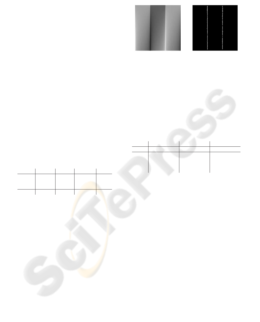
(a) (b)

Figure 1: (a) Test image representing a continuum of

phases taking values in (−π,π] corresponding to a con-

tinuum of oriented grey-level structures as expressed in a

changing “circular” manifold (cf. (Kovesi, 1999)). The

feature type changes progressively from a step edge to a

line feature, while retaining perfect phase congruency. (b)

Phase-based localization of contours obtained by the Gabor

ﬁlters.

Table 2: Accuracy evaluation for localization, phase and

orientation in the synthetic image of Figure 1. The localiza-

tion error is expressed in pixels, whereas the orientation and

phase errors are in radians.

localization orientation phase

avg std avg std avg std

Gabor 0.067 0.026 0.021 0.007 0.025 0.005

0.072 0.027 0.022 0.008 0.032 0.006

0.076 0.017 0.042 0.011 0.340 0.203

SQF

0.124 0.062 0.026 0.021 0.198 0.092

Binocular disparity. The tsukuba, sawtooth and

venus stereo-pairs from the Middlebury stereo vision

page (Scharstein and Szeliski, 2002) are used in the

evaluation. Since we are interested in the precision

of the ﬁlters we do not use the integer-based mea-

sures proposed there but instead compute the mean

and standard deviation of the absolute disparity er-

ror. To prevent outliers to distort the results, the er-

ror is evaluated only at regions that are textured, non-

occluded and continuous. The best results (see Ta-

ble 3)are obtained with the Gabor ﬁlters. Slightly

worse are the results with 4th-order steerable ﬁlters

and the 2nd-order ﬁlters yield results about twice as

bad as the 4th-order ﬁlters. The results obtained with

SQFs are comparable with those obtained by the 2nd-

order steerable ﬁlters. Figure 2 contains the left im-

ages of the stereo-pairs, the ground truth depth maps,

and the depth maps obtained with the Gabor ﬁlters.

Optic ﬂow. We have evaluated the different ﬁlters

with respect to optic ﬂow estimation on the diverg-

ing tree and yosemite sequences from (Barron et al.,

1994), using the error measures presented there. The

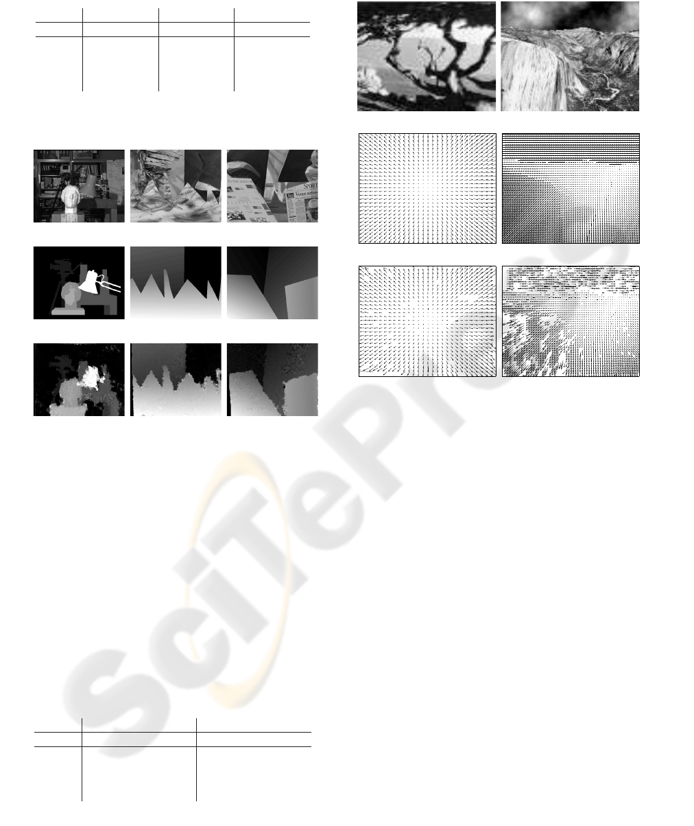
Table 3: Average and standard deviation of the absolute er-

rors in the disparity estimates (in pixels).

tsukuba sawtooth venus

avg std avg std avg std

Gabor 0.32 0.61 0.41 1.26 0.25 0.77

0.36 0.68 0.50 1.86 0.40 1.30

0.47 0.79 1.12 2.50 0.98 2.44

SQF

0.46 0.85 0.93 2.20 0.95 2.40

tsukuba sawtooth venus

Figure 2: Left frame (top row), ground truth disparity (mid-

dle row), and estimated disparity using Gabor ﬁlters (bot-

tom row).

cloud region was excluded from the yosemite se-

quence. The results are presented in Table 4 and

similar conclusions can be drawn as in the previous

Section. Gabor and 4th-order steerable ﬁlters yield

comparable results whereas 2nd-order steerable ﬁl-

ters score about twice as bad. The results obtained by

SQFs are slightly worse, since the resulting optic ﬂow

have larger errors but a higher density. Figure 3 shows

the center images, ground truth optic ﬂow ﬁelds, and

the optic ﬂow ﬁelds computed with the Gabor ﬁlters.

Table 4: Average and standard deviation of the optic ﬂow

errors (in pixels) and optic ﬂow density (in percent).

diverging tree yosemite (no cloud)

avg std dens avg std dens

Gabor 2.05 2.28 95.6 2.15 3.12 81.8

2.39 2.62 93.2 2.96 4.46 85.0

4.20 4.58 90.6 6.51 9.23 81.9

SQF

12.9 13.4 95.1 18.7 17.8 99.1

diverging tree yosemite

Figure 3: Center frame (top row), ground truth optic ﬂow

(middle row) and estimated optic ﬂow obtained with Gabor

ﬁlters (bottom row). All optic ﬂow ﬁelds have been scaled

and subsampled ﬁve times.

Motion-in-depth. Since binocular test sequences

with the ground truth and a sufﬁciently high frame

rate are not available, it has not been possible to make

quantitative comparisons. However, considering that

motion-in-depth is a ‘derived’ quantity, we expected,

that the multichannel anisotropic ﬁltering has the

same advantages over isotropic ﬁltering alike those

observed for stereo and motion processing. Qualita-

tive results obtained in real-world sequences prelimi-

narily conﬁrmed this conclusion.

5 CONCLUSIONS

Early vision processing can be reconducted to mea-

suring the amount of a particular type of local struc-

ture with respect to a speciﬁc representation space.

The choice for an early selection of features by adopy-

ing thresholding procedures, which depend on a spe-

ciﬁc and restricted environmental context, limits the

possibility of building, on the ground of such repre-

sentations, an artiﬁcial vision system with complex

functionalities. Hence, it is more convenient to base

further perceptual processes on a more general rep-

resentation of the visual signal. The harmonic repre-

sentation discussed in this paper is a reasonable rep-

resentation of early vision process since it allows for

an efﬁcient and complete representation of (spatially

and temporally) localized structures. It is character-

ized by: (1) compactness (i.e., minimal uncertainty

of the band-pass channel); (2) coverage of the fre-

quency domain; (3) robust correspondence between

the harmonic descriptors and the perceptual ‘sub-

stances’ in the various modalities (edge, motion and

stereo). Through a systematic analysis we investi-

gated the advantages of anisotropic

isotropic ﬁlter-

ing approaches for a complete harmonic description

of the visual signal. We observed that it is prefer-

able to construct a multichannel, multiorientation rep-

resentation, thus avoiding an “early condensation” of

basic features. The harmonic content is then com-

bined in the phase-orientation space at the ﬁnal stage,

only, to come up with the ultimate perceptual deci-

sions. An analysis of possible advantages of the ag-

gregation of the information in the monogenic im-

age in mid- and high-level perceptual tasks (e.g., im-

age classiﬁcation) would require further investigation,

and it is deferred to a future work.

ACKNOWLEDGEMENTS

This work results from a cross-collaborative effort

within the EU Project IST-FET-16276-2 “DrivSco”.

REFERENCES

Adelson, E., Anderson, C., Bergen, J., Burt, P., and Ogden,

J. (1984). Pyramid methods in image processing. RCA

Engineer, 29(6):33–41.

Barron, J., Fleet, D., and Beauchemin, S. (1994). Perfor-

mance of optical ﬂow techniques. Int. J. of Comp.

Vision, 12:43–77.

Bergen, J., Anandan, P., Hanna, K., and Hingorani, R.

(1992). Hierarchical model-based motion estimation.

In Proc. ECCV’92, pages 237–252.

Daugman, J. (1985). Uncertainty relation for resolution in

space, spatial frequency, and orientation optimized by

two-dimensional visual cortical ﬁlters. J. Opt. Soc.

Amer. A, A/2:1160–1169.

Diaz, J., Ros, E., Pelayo, F., Ortigosa, E., and Mota, S.

(2006). FPGA based real-time optical-ﬂow system.

IEEE Trans. Circuits and Systems for Video Technol-

ogy, 16(2):274–279.

Felsberg, M. and Sommer, G. (2001). The monogenic sig-

nal. IEEE Trans. Signal Processing, 48:3136–3144.

Fleet, D. and Jepson, A. (1993). Stability of phase in-

formation. IEEE Trans. Pattern Anal. Mach. Intell.,

15(12):1253–1268.

Fleet, D., Jepson, A., and Jenkin, M. (1991). Phase-based

disparity measurement. CVGIP: Image Understand-

ing, 53(2):198–210.

Fleet, D. J. and Jepson, A. D. (1990). Computation of com-

ponent image velocity from local phase information.

Int. J. of Comp. Vision, 1:77–104.

Freeman, W. and Adelson, E. (1991). The design and use

of steerable ﬁlters. IEEE Trans. Pattern Anal. Mach.

Intell., 13:891–906.

Gautama, T. and Van Hulle, M. (2002). A phase-based ap-

proach to the estimation of the optical ﬂow ﬁeld us-

ing spatial ﬁltering. IEEE Trans. Neural Networks,

13(5):1127–1136.

Harris, J. and Watamaniuk, S. N. (1995). Speed discrimina-

tion of motion-in-depth using binocular cues. Vision

Research, 35(7):885–896.

Kehtarnavaz, N. and Gamadia, M. (2005). Real-Time Im-

age and Video Processing: From Research to Reality.

Morgan & Claypool Publishers.

Koenderink, J. and van Doorn, A. (1987). Representation

of local geometry in the visual system. Biol. Cybern.,

55:367–375.

Kovesi, P. (1999). Image features from phase congruency.

Videre, MIT Press, 1(3):1–26.

uger, N. and Felsberg, M. (2003). A continuous formula-

tion of intrinsic dimension. In Proc. British Machine

Vision Conference, Norwich, 9-11 September 2003.

uger, N. and Felsberg, M. (2004). An explicit and com-

pact coding of geometric and structural information

applied to stereo matching. Pattern Recognition Let-

ters, 25(8):849–863.

Marr, D. (1982). Vision. New York: Freeman.

Nestares, O., Navarro, R., Portilla, J., and Tabernero, A.

(1998). Efﬁcient spatial-domain implementation of a

multiscale image representation based on Gabor func-

tions. J. of Electronic Imaging, 7(1):166–173.

Owens, R. (1994). Feature-free images. Pattern Recogni-

tion Letters, 15:35–44.

Pauwels, K. and Van Hulle, M. (2006). Optic ﬂow from

unstable sequences containing unconstrained scenes

through local velocity constancy maximization. In

Proc. British Machine Vision Conference, Edinburgh,

4-7 September 2006.

Sabatini, S., Solari, F., Cavalleri, P., and Bisio, G. (2003).

Phase-based binocular perception of motion in depth:

Cortical-like operators and analog VLSI architectures.

EURASIP J. on Applied Signal Proc., 7:690–702.

Sanger, T. (1988). Stereo disparity computation using Ga-

bor ﬁlters. Biol. Cybern., 59:405–418.

Scharstein, D. and Szeliski, R. (2002). A taxonomy and

evaluation of dense two-frame stereo correspondence

algorithms. Int. J. of Comp. Vision, 47(1–3):7–42.

Solari, F., Sabatini, S., and Bisio, G. (2001). Fast technique

for phase-based disparity estimation with no explicit

calculation of phase. Elect. Letters, 37:1382–1383.