A COMPARISION OF MODEL-BASED METHODS FOR KNEE

CARTILAGE SEGMENTATION

J. Cheong

, N. Faggian

, G. Langs

3,4

, D. Suter

and F. Cicuttini

Dept. of Electrical and Computer Systems Engineering, Monash University, Australia

Clayton School of Information Technology, Monash University, Australia

Institute for Computer Graphics and Vision, Graz University of Technology, Austria

Pattern Recognition and Image Processing Group, Vienna University of Technology, Austria

Dept. of Epidemiology and Preventive Medicine, Monash University, Australia

Keywords:

Segmentation, Model-based, Cartilage, Osteoarthritis.

Abstract:

Osteoarthritis is a chronic and crippling disease affecting an increasing number of people each year. With

no known cure, it is expected to reach epidemic proportions in the near future. Accurate segmentation of

knee cartilage from magnetic resonance imaging (MRI) scans facilitates the measurement of cartilage volume

present in a patient’s knee, thus enabling medical clinicians to detect the onset of osteoarthritis and also cru-

cially, to study its effects. This paper compares four model-based segmentation methods popular for medical

data segmentation, namely Active Shape Models (ASM) (Cootes et al., 1995), Active Appearance Models

(AAM) (Cootes et al., 2001), Patch-based Active Appearance Models (PAAM) (Faggian et al., 2006), and

Active Feature Models (AFM) (Langs et al., 2006). A comprehensive analysis of how accurately these meth-

ods segment human tibial cartilage is presented. The results obtained were benchmarked against the current

“gold standard” (cartilage segmented manually by trained clinicians) and indicate that modeling local texture

features around each landmark provides the best results for segmenting human tibial cartilage.

1 INTRODUCTION

Model-based segmentation methods have become a

standard and popular method for detecting structures

in medical images. They meet the need to consis-

tently identify landmarks on images with complex

content by the use of a priori knowledge. Active

Shape Models (ASM) (Cootes et al., 1995) and Ac-

tive Appearance Models (AAM) (Cootes et al., 2001)

have proven to provide reliable localisation of land-

marks.

ASM is based on building a statistical shape

model for a given class of objects. Since its introduc-

tory application for segmenting heart ventricles from

echocardiogram, ASM has undergone many modiﬁ-

cations and found numerous new applications for seg-

menting medical images. Some examples include

segmenting lungs from chest radiographs (van Gin-

neken et al., 2001), metacarpal bone from hand ra-

diographs (Langs et al., 2003), and human knee car-

tilage from MRI scans (Cheong et al., 2005). The

concept of ASM was extended to include a model of

the object’s texture and this new method was termed

Active Appearance Models, AAM. Common uses of

AAM these days include segmenting brain structure

from brain MRI and heart ventricles from cardiac

MRI (Oost et al., 2003).

Recent modiﬁcations to speed up AAM have re-

sulted in methods that model only relevant parts of

an object’s texture instead of the entire texture. For

example, Patch-based AAM (PAAM) (Faggian et al.,

2006) model a texture patch oriented along each land-

mark, while Active Feature Models (AFM) (Langs

et al., 2006), represent image texture by means of lo-

cal texture descriptors. These methods produce re-

sults similar to or better than AAM even with a sig-

niﬁcantly reduced amount of training information.

The motivation behind this study is to identify

a model-based segmentation method that can ac-

curately and efﬁciently segment human tibial carti-

lage, with the ultimate goal being a fully automated

method. Accurate segmentation enables the carti-

lage volume of a patient to be estimated, and stud-

ies have shown that such measures will enable eval-

uation of osteoarthritis severity in the knee (Cicuttini

et al., 2003; Raynauld, 2002). The current method

290

Cheong J., Faggian N., Langs G., Suter D. and Cicuttini F. (2007).

A COMPARISION OF MODEL-BASED METHODS FOR KNEE CARTILAGE SEGMENTATION.

In Proceedings of the Second International Conference on Computer Vision Theory and Applications - IFP/IA, pages 290-295

 SciTePress

of cartilage volume measurement involves some form

of manual segmentation performed by a trained clin-

ician; and the process is slow, tedious, and subjec-

tive. There is thus a strong demand to develop a non-

subjective and more efﬁcient segmentation method

to meet the needs of large-scale clinical trials and

epidemiological studies that have been conducted to

evaluate therapies that may slow down or stop carti-

lage degradation.

This paper is organised as follows. In Section 2,

we describe the four model-based segmentation meth-

ods used. In Section 3, the experimental setup is ex-

plained and the results are presented and discussed.

Concluding remarks are given in Section 4.

2 METHODS

2.1 Active Shape Models

Active Shape Models (ASM) (Cootes et al., 1995) is a

model-based segmentation technique that models the

variation of object shape in images. Objects are repre-

sented as a set of n labeled points referred to as land-

marks. The locations of these landmarks are extracted

either manually or automatically from a set of p train-

ing images. In the segmentation process, the algo-

rithm searches for the best candidate points for each

landmark in the image based on local edge features,

with the solution space constrained by a global shape

model.

The shape model is constructed by stacking the

landmarks (x

,...x

) for each training image

into a shape vector, s

= (x

,...x

)

. (1)

The shape vectors are aligned by scaling, rotation and

translation using an iterative scheme known as Gen-

eralised Procrustes Analysis (GPA) (Goodall, 1991)

to minimise the sum of squared distances between the

landmarks. A mean shape, ¯s, is then calculated from

the shape vectors s,

¯s =

∑

i=1

, (2)

as well as the covariance matrix,

C =

p−1

∑

i=1

− ¯s)(s

− ¯s)

. (3)

Principal component analysis (PCA) is then applied

using eigenvalue decomposition of the covariance

matrix. Eigenvectors corresponding to the r largest

eigenvalues λ

are retained in a matrix S. The number

of eignevalues to retain, r, is chosen such that their

sum sufﬁciently explains the variance in the training

shapes, since the variance explained by each eigen-

vector is equal to the corresponding eigenvalue. r

is usually set such that the explained variance ranges

from 90% to 99.5%. Any shape in the training set can

now be approximated by:

ˆs = ¯s+ Sα, (4)

where α is a vector of r elements containing the shape

coefﬁcients, calculated by:

α = S

( ˆs− ¯s). (5)

To ensure that new shapes generated are in the al-

lowable shape domain, the values of α are constrained

to lie within the range ±m

√

, where m has a value

between 2 and 3.

The shape model is ﬁtted onto an image by placing

the mean shape, with shape coefﬁcients initialised to

0, onto an initial location. The neighborhood of each

landmark of the initial ﬁt is then examined to ﬁnd bet-

ter locations for the ﬁtting. This is implemented by

examining the normals along each landmark for the

strongest edge. The shape and pose of the ﬁt is then

updated, constrained by limits set to the variation of

α. This procedure is iterated until convergence, i.e.

there is no signiﬁcant change in shape between two

consecutive iterations.

There are many different improvements that have

been made to ASMs, these usually deal with dif-

ferent implementations of better landmark position

searches. The most common improvement is to build

some form of texture model around each landmark

(van Ginneken et al., 2001; Yan et al., 2002), very

much like PAAM, discussed in Section 2.3. This ex-

tra model is claimed to produce more accurate land-

mark localisation compared to searching only for the

strongest edge.

2.2 Active Appearance Models

Active Appearance Model (AAM) (Cootes et al.,

2001) is a more powerful and more computer-

intensive model based segmentation technique. Un-

like ASM, it models two principle modes of object

variation in images, shape and texture. The idea

behind AAM is to improve segmentation results by

modeling the complete texture of an object. AAM

uses a ﬁxed number of landmarks to represent objects

and encodes shape variation much like ASM.

The texture variation of an object is modeled in a

similar fashion. In the texture model, GPA is replaced

with an object transformation step. Here, objects are

transformed to the mean coordinate frame. This mean

is provided by the shape model in equation (4). PCA

is then applied to the aligned objects to form a simple

linear representation for a novel texture,

t =

t + Tγ, (6)

where

t is the mean texture, T is a linear combination

of the orthogonal subspace of textures, and γ consists

of the texture coefﬁcients. By combining these tex-

ture and shape models, it is possible to render a novel

image:

I(α,γ) = F( ¯s+ Sα,

t + Tγ). (7)

Rendering is deﬁned as the process of transform-

ing a generated texture to ﬁt a desired shape. The

texture exists in a shape free representation and is

bi-linearly re-sampled (F) to the desired shape using

a piecewise afﬁne transformation. The shape model

is triangulated and these triangles are transformed to

the mean coordinate frame through a series of afﬁne

transformation, different for each triangle. The search

process now involves ﬁtting the texture and shape

model to the image. This is a non-linear optimisation

task and there are many strategies to implement this.

For this paper, Inverse Compositional Image Align-

ment (ICIA) was used for AAM ﬁtting (Faggian et al.,

2005). This approach minimises the difference, e, be-

tween the mean AAM template and the image:

e =

∑

−I(W(x;α))]

, (8)

where A

is the mean shape and mean texture that

AAM renders and I(W(x;α)) is the image sampled

to the mean shape coordinate frame using the shape

coefﬁcients α.

2.3 Patch-based Active Appearance

Models

Patch-based AAM (PAAM) (Faggian et al., 2006) is

a modiﬁcation to AAM. It differs from AAM in the

way it samples texture in images. Instead of using

triangulation, PAAM makes use of oriented patches

centered on each landmark. An oriented patch is de-

ﬁned at each landmark location by the shape model’s

connectivityusing its two adjacent landmarks. For ex-

ample, the second landmark in a model, v

and its ad-

jacent landmarks, v

and v

are used to deﬁne a patch

about v

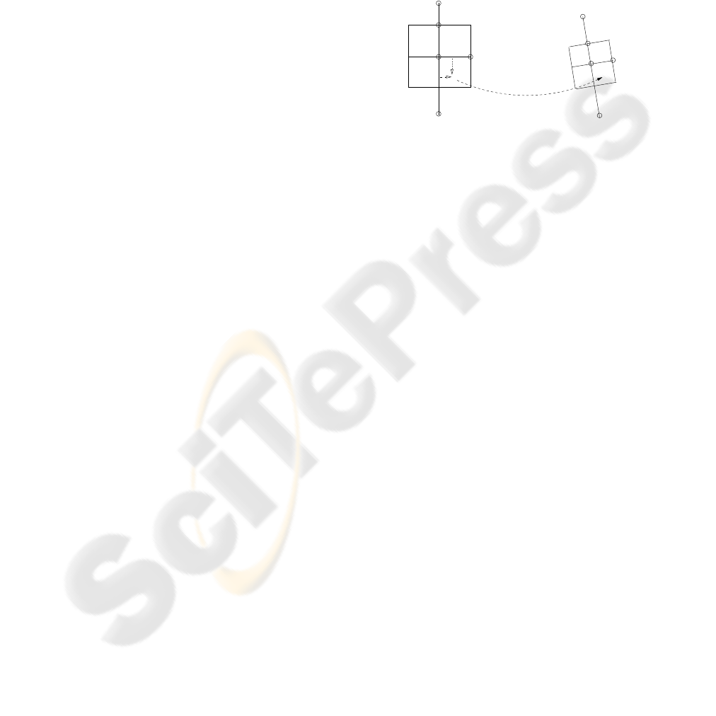
. A patch is now constructed by computing

two principle directions. The ﬁrst principle direction

is the normal of v

to v

, called u

⊥

. The second prin-

ciple direction is orthogonal to the ﬁrst and is called

u. These principle directions can be used to transform

pixels from one patch into another using Barycentric

coordinates, an example is shown in Figure 1.

The size of each patch is deﬁned by a constant,

k. This constant must be suitably selected by the user

during PAAM construction. In practice, a larger k in-

creases the robustness of the method with respect to

alignment errors while a smaller k increases conver-

gence when alignment is known to be good. The ﬁt-

ting process for PAAM is similar to AAM; ICIA is

used to minimise the difference, e, between the mean

AAM template and the patch-sampled image.

⊥

ˆv

ˆu

⊥

ˆv

ˆu

ˆx = ˆv

+ α(ˆu − ˆv

) + β(ˆu

⊥

− ˆv

)

ˆx

Figure 1: Transforming a pixel, x, in patch deﬁned by v

, v

to its corresponding position, ˆx, in a different patch

deﬁned by ˆv

, ˆv

, (Faggian et al., 2006).

2.4 Active Feature Models

Active Feature Models (AFM) (Langs et al., 2006)

build a model based on a set of training images for

which corresponding positions of a set of landmarks

are known. A statistical shape model is built based on

the training shapes, much like ASM. Instead of mod-

eling local texture around the landmarks directly, as

in PAAM, AFM compacts the local texture by feature

extraction using descriptors. In addition, AFM does

not use landmark connectivity like PAAM, thus de-

scriptors are independent of the shape’s contour di-

rection. Any descriptor can be used, allowing for

straightforward adaptation of the algorithm to dif-

ferent data, especially if descriptors with favorable

speciﬁcity and robustness with respect to the appli-

cation are known.

During training, model parameters are perturbed

randomly generating a large number of displaced

model instances. A functional relation is then learned

from the resulting feature vectors f describing lo-

cal texture and the corresponding parameter displace-

ment δp by Canonical Correlation Analysis (CCA).

This is analogous to a CCA based AAM search ap-

proach proposed in (Donner et al., 2006).

The AFM search process involves extracting local

texture features at the current landmark position esti-

mates and updating the model parameters according

to the trained relation

3 EXPERIMENTS

3.1 Setup

Experimental results are reported for two datasets,

medial tibial cartilage and lateral tibial cartilage. Car-

tilage boundaries segmented by Operator 1 in July

2005 were used as the baseline “gold standard” mea-

sures for all experiments as this was the only dataset

available to us until recently. Manual segmentations

carried out as followup tests by Operators 1 and 2

in September 2006 provide target benchmarks. From

our database of “gold standard” cartilage outlines, we

randomly selected 5 patients, totalling 78 medial and

87 lateral image slices. Correspondences of 32 land-

marks for images of each dataset were obtained using

a Minimum Description Length (MDL) shape algo-

rithm (Thodberg, 2003). 5-fold cross-validation was

performed on the datasets for ASM, AAM, PAAM

and AFM to compare segmentation results.

All methods were initialised with the true center

of gravity (CoG) of the corresponding cartilage, cal-

culated by ﬁnding the mean of the 32 landmark lo-

cations. An optimal normal length of 3 was used

to search for landmark positions with ASM. For the

PAAM experiments, the patch size, k, was set to 14

and for the AFM experiments, steerable ﬁlters (Free-

man and Adelson, 1991) were used due to their reli-

ability and low dimensionality. A gabor jet with ﬁl-

ter frequency φ = 1 and directions θ ∈ {π/2,3π/4}

proved to give the best descriptions for cartilage seg-

mentation.

The following measures were employed to com-

pare the different segmentation results, Goodness of

Fit (GOF), sensitivity, and the difference in area be-

tween the segmentation results and the “gold stan-

dard”. The GOF measure is deﬁned as:

GOF =

TP+ FP+ FN

, (9)

where TP represents true positive (segmented area

correctly classiﬁed as cartilage), FP represents false

positive (segmented area incorrectly classiﬁed as car-

tilage), and FN represents false negative (cartilage

area incorrectly classiﬁed as background). A GOF of

1 represents a perfect overlap with the “gold standard”

and a GOF of 0 represents no overlap with the “gold

standard”. Sensitivity is deﬁned:

Sensitivity =

No. of pixels in “gold standard” seg.

. (10)

Sensitivity measures the proportion of the “gold stan-

dard” that is segmented and provides a useful indica-

tion of oversegmentation or undersegmentation when

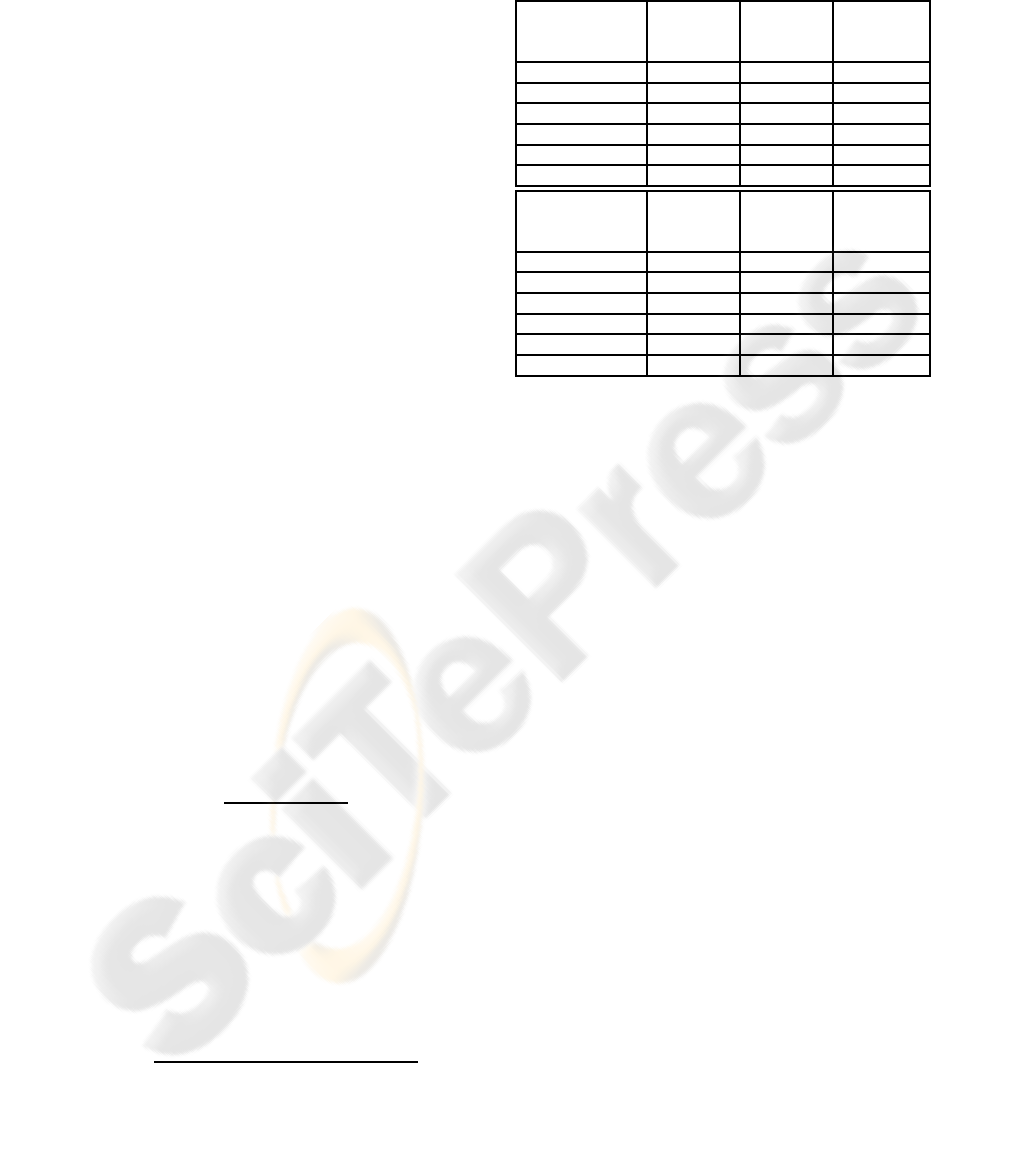
Table 1: Mean and standard deviation results of the Good-

ness of Fit (GOF), sensitivity, and difference in area when

compared to the “gold standard” for different segmentation

methods.

Medial Tibial GOF Sensitivity Area Diff.

Cartilage µ ± σ µ ± σ (mm

)

µ ± σ

ASM 0.60 ± 0.14 0.74 ± 0.14 10.27 ±7.85

AAM 0.41 ± 0.15 0.56 ± 0.20 21.31 ±14.22

PAAM 0.64 ± 0.15 0.74 ± 0.13 9.95 ± 7.38

AFM 0.54 ± 0.11 0.69 ± 0.10 9.08 ± 7.27

Manual Operator 1 0.82 ± 0.07 0.89 ± 0.06 3.47 ± 2.79

Manual Operator 2 0.79 ± 0.09 0.88 ± 0.08 5.17 ± 4.42

Lateral Tibial GOF Sensitivity Area Diff.

Cartilage µ ± σ µ ± σ (mm

)

µ ± σ

ASM 0.60 ± 0.16 0.74 ± 0.17 18.68 ±16.85

AAM 0.48 ± 0.13 0.61 ± 0.19 30.35 ±20.27

PAAM 0.72 ± 0.09 0.79 ± 0.10 15.76 ±14.50

AFM 0.54 ± 0.20 0.69 ± 0.20 17.65 ±17.77

Manual Operator 1 0.85 ± 0.06 0.92 ± 0.05 3.09 ± 2.67

Manual Operator 2 0.80 ± 0.08 0.88 ± 0.06 4.92 ± 3.64

combined with the GOF measure. GOF and sensitiv-

ity provide a measure of the segmentation accuracy

while the area difference provides an estimation of

measurement accuracy.

3.2 Results

The results of all experiments are given in Table 1,

and Figures 2 and 3 showtypical result for each exper-

iment. PAAM produces the best segmentation results

for both medial and lateral tibial cartilage. It is the

only method from the four that models background

texture locally around the landmarks, taking into ac-

count the connectivity of the landmarks. The tex-

ture patch model includes both foreground and back-

ground, thus enabling PAAM to correctly locate the

cartilage boundaries with higher success.

AAM produces the worst results because it mod-

els only the texture within the cartilage. This leads to

poor performance because there is inherently a large

variation in texture due to the biochemically hetero-

geneous property of cartilage. Without modeling any

background information, it is difﬁcult for AAM to lo-

cate the cartilage boundaries.

AFM produces reasonable results even though the

data in Table 1 ranks AFM as third best behind ASM

and PAAM. The segmented shapes of PAAM and

AFM are smoother than ASM and examples can be

observed in Figures 2 and 3. Background texture is

not used directly by AFM but represented by means

of features extracted by descriptors using steerable ﬁl-

ters. AFM tends to oversegment images because the

ﬁlter blurs the edges of the cartilage, thus making it

harder to locate the correct boundary.

Figure 2a displays a common problem that ASM

exhibits. Landmarks are attracted to regions with

strong edges, therefore in slices where the tibial and

femoral cartilage touch, there is no edge information

for the upper boundary of the tibial cartilage and ASM

locates the upper boundary of the femoral cartilage

instead. The resulting shape estimate from ASM also

tends to be uneven, compared to PAAM and AFM.

This is because when new landmark locations are

found, the pose and shape parameters are updated to

best match the shape model to these landmark points.

This step can potentially shift the shape model away

from the true landmark positions.

All methods perform very poorly on a few par-

ticular slices, namely slices located at the very ends

of the cartilage in the middle of the knee. On these

slices, the cartilage areas are very small and also dis-

play very poor contrast and high shape variability.

Even the manual operators exhibit some discrepancy

in their results for these slices.

4 CONCLUSION

In this paper, we have compared four different model-

based segmentation methods (ASM, AAM, PAAM

and AFM) for the purpose of tibial cartilage segmen-

tation. All four methods have been ﬁne tuned so that

only the optimal settings for cartilage segmentation

were compared. In conclusion, methods that work on

local texture perform better for cartilage segmentation

due to a restriction to more relevantinformation being

used for regression and ﬁtting. In addition, the use of

landmark connectivity for orientation consistency re-

sults in an even more speciﬁc description of the tex-

ture.

ACKNOWLEDGEMENTS

The authors would like to thank Fahad Hanna and

Yuanyuan Wang for their time and contribution with

performing the manual cartilage segmentation used in

this paper, and also Ren´e Donner for providing parts

of the AFM implementation. Georg Langs has been

supported by the Austrian Science Fund(FWF) under

the Grant P17083-N04 (AAMIR).

REFERENCES

Cheong, J., Suter, D., and Cicuttini, F. (2005). Development

of semi-automatic segmentation methods for measur-

ing tibial cartilage volume. In Proc. DICTA 2005,

pages 307–314.

Cicuttini, F., Wluka, A. E., Forbes, A., and Wolfe, R.

(2003). Comparison of tibial cartilage volume and ra-

diologic grade of the tibiofemoral joint. Arthritis and

Rheumatism, 48:682–688.

Cootes, T., Edwards, G., and Taylor, C. (2001). Active ap-

pearance models. IEEE TPAMI, 23(6):681–685.

Cootes, T., Taylor, C., Cooper, D., and Graham, J. (1995).

Active shape models - their training and application.

Computer Vision and Image Understanding, 61(1).

Donner, R., Reiter, M., Langs, G., Peloschek, P., and

Bischof, H. (2006). Fast active appearance model

search using canonical correlation analysis. IEEE

TPAMI, 28(10):1690 – 1694.

Faggian, N., Paplinski, A., and Sherrah, J. (2006). Local

texture patches for active appearance models. In Proc.

IVCNZ 2006.

Faggian, N., Romdhani, S., Paplinski, A., and Sherrah, J.

(2005). Color active appearance model analysis using

a 3d morphable model. In Proc. DICTA 2005, pages

407–414.

Freeman, W. T. and Adelson, E. H. (1991). The design and

use of steerable ﬁlters. IEEE TPAMI, 13(9):891–906.

Goodall, C. (1991). Procrustes methods in the statistical

analysis of shapes. Journal of the Royal Statistical

Society, 53:285–339.

Langs, G., Peloschek, P., and Bischof, H. (2003). Asm

driven snakes in rheumatoid arthritis assessment. In

Proc. SCIA 2003, pages 454–461.

Langs, G., Peloschek, P., Donner, R., Reiter, M., and

Bischof, H. (2006). Active feature models. In Proc.

ICPR 06,, volume 1, pages 417–420.

Oost, C. R., Lelieveldt, B. P. F.,

Uz¨umc¨u, M., Lamb, H. J.,

Reiber, J. H. C., and Sonka, M. (2003). Multi-view

active appearance models: Application to x-ray lv an-

giography and cardiac mri. In IPMI 2003, pages 234–

245.

Raynauld, J. (2002). Magnetic resonance imaging of ar-

ticular cartilage: toward a redeﬁnition of ”primary”

knee osteoarthritis and its progression. The Journal of

Rheumatology, 29:1809–1810.

Thodberg, H. (2003). Minimum description length shape

and appearance models. In IPMI 2003, pages 51–62.

van Ginneken, B., Frangi, A. F., Staal, J., ter Haar Romeny,

B. M., and Viergever, M. A. (2001). A non-linear

gray-level appearance model improves active shape

model segmentation. In Proc. MMBIA 2001, pages

117–127. IEEE Computer Society Press.

Yan, S., Liu, C., Li, S., Zhang, H., Shum, H.-Y., and Cheng,

Q. (2002). Texture-constrained active shape models.

In Proc. GMBV 2002, pages 107–113.

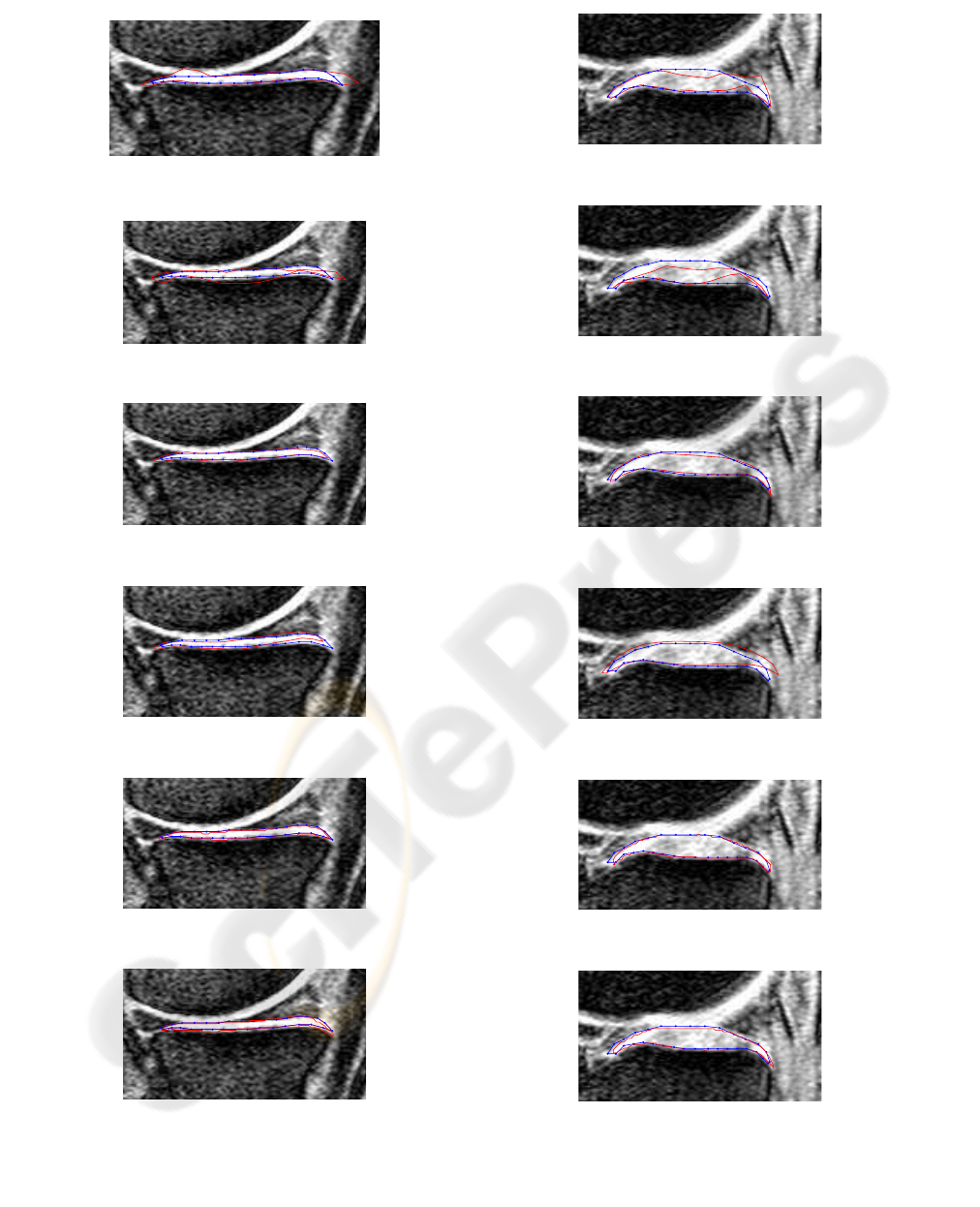
(a) ASM

GOF = 0.70, Sens = 0.92, Area Diff. = 11.43mm

(b) AAM

GOF = 0.53, Sens = 0.76, Area Diff. = 10.94mm

GOF = 0.77, Sens = 0.87, Area Diff. = 0.78mm

(d) AFM

GOF = 0.59, Sens = 0.70, Area Diff. = 0.92mm

(e) Manual Operator 1

GOF = 0.88, Sens = 0.94, Area Diff. = 0.68mm

(f) Manual Operator 2

GOF = 0.79, Sens = 0.91, Area Diff. = 4.54mm

Figure 2: Example results for medial tibial cartilage. Seg-

mentations are given by the solid line and the “gold stan-

dard” by the dotted line. NOTE: Images are best viewed in

colour.

(a) ASM

GOF = 0.65, Sens = 0.72, Area Diff. = 16.70mm

(b) AAM

GOF = 0.43, Sens = 0.44, Area Diff. = 51.56mm

GOF = 0.79, Sens = 0.82, Area Diff. = 13.28mm

(d) AFM

GOF = 0.69, Sens = 0.86, Area Diff. = 15.72mm

(e) Manual Operator 1

GOF = 0.92, Sens = 0.95, Area Diff. = 1.42mm

(f) Manual Operator 2

GOF = 0.88, Sens = 0.90, Area Diff. = 7.08mm

Figure 3: Example results for lateral tibial cartilage. Seg-

mentations are given by the solid line and the “gold stan-

dard” by the dotted line. NOTE: Images are best viewed in

colour.