
MOTION BLUR ESTIMATION AT CORNERS
Giacomo Boracchi and Vincenzo Caglioti
Dipartimento di Elettronica e Informazione, Politecnico di Milano, Via Ponzio, 34/5- 20133 MILANO
Keywords:
Point Spread Function Parameter Estimation, Motion Blur, Space Varying Blur, Blurred Image Analysis,
Optical Flow.
Abstract:
In this paper we propose a novel algorithm to estimate motion parameters from a single blurred image, ex-
ploiting geometrical relations between image intensities at pixels of a region that contains a corner. Corners
are significant both for scene and motion understanding since they permit a univocal interpretation of motion
parameters. Motion parameters are estimated locally in image regions, without assuming uniform blur on im-
age so that the algorithm works also with blur produced by camera rotation and, more in general, with space
variant blur.
1 INTRODUCTION
Motion estimation is a key problem both in image
processing and computer vision. It is usually per-
formed comparing frames from a video sequence or a
pair of still images. However, in case of fast motion or
long exposure images, motion can be also estimated
by analyzing only a single blurred image. Algorithms
that consider one image have to face a more challeng-
ing problem, because little information is available,
since both image content and blur characteristics are
unknown.
In this paper we introduce an algorithm to estimate
motion from a single blurred image, exploiting mo-
tion direction and length at image corners. Several
algorithms that estimate motion blur from a single im-
age have been proposed; most of them process the im-
age Fourier transform, assuming uniform blur (Choi
et al., 1998), (Kawamura et al., 2002). Rekletis (Rek-
leitis, 1996) estimates locally motion parameters from
a blurred image by defining an image tessellation, and
then analyzing Fourier transform of each region sep-
arately. However frequency domain based algorithms
are not able to manage blur when motion parame-
ters are varying through the image. Moreover, motion
estimation from Fourier domain is particularly diffi-
cult at image corners because Fourier coefficients are
mostly influenced by the presence of edges than from
blur.
Our algorithm considers image regions containing a
blurred corner and estimates motion direction and
length by exploiting geometrical relations between
pixels intensity values. Beside blind deconvolution,
motion estimation from a single image has been ad-
dressed for several other purposes. Rekleitis estimates
the optical flow (Rekleitis, 1996), Lin determines ve-
hicle and ball speed (Lin and Chang, 2005), (Lin,
2005) and more recently Klein (Klein and Drum-
mond, 2005) suggested a visual gyroscope based on
estimation of rotational blur.
The paper is organized as follows: in Section 2 the
blur model and the corner model are introduced, in
Section 3 we present the algorithm core idea and in
Section 4 we describe a robust solution based on a
voting algorithm. Section 5 describes the algorithm
details and presents experimental results.
2 PROBLEM FORMULATION
Our goal is to estimate blur direction and extent at
some salient points, which are pixels where it is pos-
sible to univocally interpret the motion. For exam-
ple, pixels where the image is smooth as well as
296
Boracchi G. and Caglioti V. (2007).
MOTION BLUR ESTIMATION AT CORNERS.
In Proceedings of the Second International Conference on Computer Vision Theory and Applications - IFP/IA, pages 296-302
Copyright
c
SciTePress
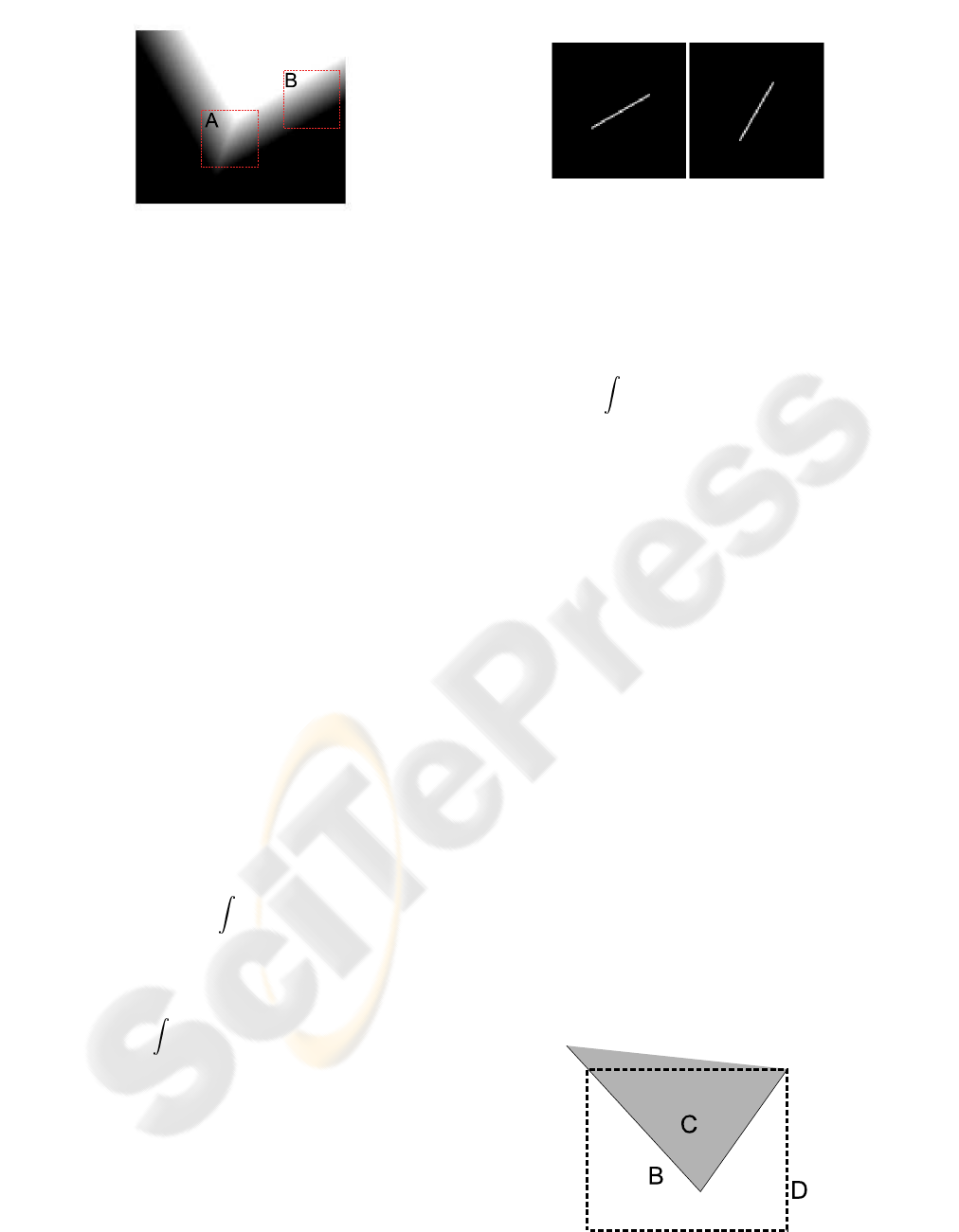
Figure 1: Blurred corner synthetically generated.
pixels along a blurred edge do not allow an univo-
cal motion interpretation: given a blurred edge or
a blurred smooth area there are potentially infinite
scene displacements that could have caused the same
blur (see region B in Figure 1). Corners, instead, offer
a clear interpretation of motion direction and extent
and that’s the reason why we design an algorithm to
estimate motion specifically at corners. We consider
image I modelled as follows
I(x) = K
y+ ξ
(x) + η(x), x = (x
1
,x
2
) (1)
where x is a multi index representing image coordi-
nates varying on a discrete domain X, y is the original
and unknown image and K is the blur operator. We
introduce two different sources of white noise, ξ and
η. In our model η represents electronic and quanti-
zation noise, while ξ has been introduced to attenuate
differences between corners in real images and the bi-
nary corner model that we present in the next section.
Therefore ξ plays a crucial role only when a region
containing a corner is analyzed.
2.1 The Blur Model
Here we model the blur operator K on the whole im-
age, so that we do not need to consider ξ which is
relevant only at image corners.
Our goal is to determine the blur operator K which
can be written as (Bertero and Boccacci, 1998)
K
y
(x) =
X
k(x,µ)y(µ)dµ. (2)
Usually, K is considered space invariant, so that equa-
tion (2) becomes a convolution with a kernel v, called
point spread function (PSF)
K
y
(x) =
X
v(x− µ)y(µ)dµ = (v⋆ y)(x). (3)
This assumption is too restrictive for our purpose, be-
cause often scene points follow different trajectories
with respect to the camera viewpoint and are indeed
differently blurred. Equation (3) does not concern,
for instance, scenes where there are objects following
different trajectories, scenes with a moving target on
a still background and static scenes captured by a ro-
tating camera.
Figure 2: Example of motion blur psf with direction 30 and
60 degrees respectively and length 30 pixels.
On the other hand, solving (2) is a difficult inverse
problem: to reduce its complexity we assume that the
blur functional K is locally approximated as a shift in-
variant blur, i.e.
∀x
0
∈ X, ∃U
0
⊂ X , x
0
∈ U
0
and a PSF v
0
such that
K
y
(x) ≈
X
v
0
(x− µ)y(µ)dµ ∀x ∈ U
0
. (4)
Furthermore, we consider only motion blur PSF
defined over an 1-D linear support: they can be writ-
ten as
v
0
= R
(θ)
s
l
(x) θ ∈ [0,2π],l ∈ N
s
l
(x
1
,x
2
) =
1/(2l + 1), −l ≤ x
1
≤ l
x
2
= 0
0, else
where θ and l are motion direction and length respec-
tively and R
(θ)
s
l
is function s
l
rotated by θ degrees
on X . Figure 2 shows examples of motion blur PSF.
2.2 The Corner Model
Our corner model relies on two assumptions. Firstly,
we assume that y is a grayscale image or, equivalently,
an image plane in a color representation which is con-
stant at corner pixels and at background pixels. This
means that given D ⊂ X, neighborhood of an image
corner, we have y(D) = {b,c}, where b and c are the
image values for the background and for the corner,
respectively. Moreover, the sets of pixels belonging
to the background B = y
−1
({b}) and the set of pix-
els belonging to the corner C = y
−1
({c}), have to be
separated by two straight segments (having a common
endpoint). Figure 3 shows the corner model.
Then, let us define ˜v as the corner displacement vec-
Figure 3: The Corner Model.
tor: this vector has the origin at image corner and di-
rection θ and length l equal to direction and length of
the PSF v
0
which locally approximates the blur oper-
ator. Let γ be the angle between a reference axis and
the corner bisecting line, let α be the corner angle,
and θ be the angle between ˜v and the reference axis,
then
θ ∈ [γ − α/2,γ+ α/2] + kπ k ∈ N.
Figure 4.a shows a corner displacement vector satis-
fying this assumption, while Figure 4.b a corner that
does not.
α
2
θ
γ
˜v
α
2
θ
γ
˜v
a
b
Figure 4: Two possible cases for corner displacements, a
agrees with our model while b does not.
3 PROBLEM SOLUTION
In this section we derivethe core equations for motion
estimation at a blurred corner that satisfies assump-
tions of Sections 2.1 and 2.2.
We first consider noise η only, then we exploit how ξ
corrupts the proposed solution.
3.1 Binary Corners
Let us examine an image region containing a binary
corner, like the one depicted in Figure 3, and let us
assume that noise ξ is null. Let d
1
and d
2
be the first
order derivative filters w.r.t. x
1
and x
2
. The image
gradient is defined as
∇I(x) =
I
1
(x)
I
2
(x)
= ∇K
y
(x) + ∇η(x),
where I
1
= (I ⋆ d
1
) and I
2
= (I ⋆ d
2
).
If ∆ = |c − b| is the image intensity difference be-
tween the corner and the background, it follows, as
illustrated in Figure 5, that
∆ = ˜v · ∇K
y
(x), ∀x ∈ D
0
, (5)
where D
0
= {x ∈ D|∇K
y
(x) 6= [0,0]
T
}.
Equation (5) is undeterminate as we do not know ∆
and K
y
but only I, which is corrupted by η.
Similar situations can be solved taking into account,
∀x ∈ D
0
, several instances of (5), evaluated at neigh-
boring pixels.
∆
∇I
∇I
˜v
Figure 5: Intensity values of in box A of Figure 1.
We call w a window described by its weight w
i
,−n <
i < n, and we solve the following system
A(x) ˜v = ∆[w
−n
,...,w
0
,...,w
n
]
T
(6)
where A is defined as
A(x) =
w
−n
∇I(x
−n
)
T
...
w
0
∇I(x)
T
...
w
n
∇I(x
n
)
T
.
In our experiment we choose w as a squared window
having gaussian distributed weights.
A solution of system (6) is given by ˜v
˜v = argmin
v
A(x)v− ∆[w
−n
,...,w
0
,...,w
n
]
T
2
(7)
which yields
˜v = H
−1
(x)A
T
(x) [w
−n
,...,w
0
,...,w
n
] (8)
H =
∑
i
w
2
i
I
1
(x
i
)
2
∑
i
w
2
i
I
2
(x
i
)I
1
(x
i
)
∑
i
w
2
i
I
2
(x
i
)I
1
(x
i
)
∑
i
w
2
i
I
2
(x
i
)
2
.
H corresponds to Harris Matrix (Harris and Stephens,
1988), whose determinant and trace are used as cor-
ner detectors in many feature extraction algorithms,
see (Mikolajczyk et al., 2005).
If w does not contain any image corner, H is singu-
lar and consequently the system (8) does not admit
a unique solution. Therefore, when the window w in-
tersects only one blurred edge (like region B in Figure
1), system (8) admits an infinite number of solutions
and the motion parameters can not be estimated.
On the contrary, H is nonsingular when w intersects
two blurred edges (like box A in Figure 1) and in this
case the system (8) can be univocally solved.
The least square solution (8) performs optimally in
case of gaussian white noise. Here we assume that
η is white noise, without specifying any distribution
because ∇η would not be white anymore. However,
in case of noise with standard deviation significantly
smaller than ∆, equation (8) represent a suboptimal
solution.
3.2 Noisy Corners
The proposed algorithm works when y contains a
binary corner, that takes only two intensity values.
These cartoon world corners are far from being simi-
lar to corners of real images. It is reasonable to expect
corners to be distinguishable from their background,
but hardly they would be uniform. More often their
intensity values would be varying, for example, as
there are texture or details. However, since the ob-
served image I is blurred, we do not expect a big dif-
ference between a blurred texture and a blurred white
noise ξ, added on a blurred corner.
Let then consider how equation (5) changes if ξ 6= 0.
We have
∇I(x) = ∇K
y
(x) + ∇K
ξ
(x),
and (5) holds for ∇K
y
(x), while it does not for
∇K
ξ
(x).
However the blur operator K
ξ
, which is locally
a convolution with a PSF, produces a correlation of
ξ samples along the motion direction (Yitzhaky and
Kopeika, 1996), so that
∇K
ξ
(x) · ˜v ≈ 0, (9)
which means that the more blur induces correlation
among random values of ξ, the more our algorithm
will work with corners which are not binary.
4 ROBUST SOLUTION
Although the equation (9) assures that the proposed
algorithm would work for most of pixels, even in pres-
ence of noise ξ, we expect that outliers would heavily
influence the solution (8), since it is an ℓ
2
norm min-
imization (7).
Beside pixels where ∇K
ξ
(x) · ˜v 6= 0 there could be
several other noise factors that are not considered in
our model but that we should be aware of. For exam-
ple compressed images often present artifacts at edges
such as aliasing and blocking, corners on y are usually
smoothed and edges are not perfectly straight lines.
However, if we assume that outliers are a relatively
small percentage of pixels, we can still obtain a reli-
able solution using a robust technique.
We do not look for a vector ˜v that satisfy the equa-
tion (5) at each pixel or that minimize the ℓ
2
error
norm (7): rather we look for a value of ˜v that sat-
isfies a significant percentage of equations in system
(6), disregarding how ˜v is far from the solution of the
remaining equations.
4.1 The Voting Approach
If we define, for every pixel, the vector N(x) as
N(x) =
∇I(x)
||∇I(x)||
2
∆, (10)
we have that N(x) corresponds to the ˜v component
along ∇I(x) direction, ∀x ∈ D
0
.
The endpoint of any vector ˜v, solution of (5), lies on
the straight line perpendicular to N(x), going through
its endpoint. Then, the locus ℓ
x
(u) of the possible ˜v
endpoints, compatible with a given datum ∇I(x), is a
line (see Figure 6).
As in usual Hough approaches, the 2-D parameter
space of ˜v endpoints is subdivided into cells of
suitable size (e.g. 1 pixel); a vote is assigned to any
cell that contains (at least) a value of ˜v satisfying
an instance of equation (5). The most voted cells
represent values of ˜v that satisfy a significant number
of equations (6).
4.2 Neighborhood Construction
In order to reduce the approximation errors due to the
discrete parameter space and to take into account ∇η,
we assign a full vote (e.g 1) to each parameter pairs
that solve (5), (the line of Figure 6), and a fraction of
vote to the neighboring parameter pairs.
We define the following function
ℓ(u
1
,u
2
) = exp
h
−
u
2
1+ k|u
1
|σ
∇η
2
i
, (11)
ℓ
x
(u)
N(x)
u
1
u
2
Figure 6: ℓ(x) set of possible endpoint for ˜v.
where σ
∇η
is ∇η standard deviation and k is a
tuning parameter. ℓ has the following proper-
ties: it is constant and equal to 1 on u
1
axis,
(i.e. ℓ(u
1
,0) = 1), and when evaluated on a ver-
tical line, (u
1
= const), it is a gaussian function
having standard deviation that depends on |u
1
|, i.e.
ℓ(u
1
,u
2
) = N(0,1+ k|u
1
|σ
∇η
)(u
2
).
We select this function as a prototype of the vote map,
given ∇I(x), the votes distributed in the parameter
space are the values of an opportunely translated and
scaled version of ℓ(u
1
,u
2
). The straight line of Figure
6, ℓ
x
(u), is therefore replaced by function ℓ rotated by
(
π
2
− θ) degrees and translated so that its origin is in
N(x) endpoint, i.e.
ℓ
x
(u) = R
(
π
2
−θ)
ℓ
(u− N(x)), (12)
where θ is ∇I(x) direction and R
(
π
2
−θ)
is the rotation
of (
π
2
− θ) degrees.
In such a way, we give a full vote to parameter pairs
which are exact solutions of (5) and we increase the
spread of votes as the distance from N(x) endpoint in-
creases.
Figure 7(a) shows how votes are distributed in pa-
rameter space for a vector N(x). Figure 7(b) shows
parameter space after having assigned all votes, the
arrow indicates the vector ˜v estimated.
(a)
˜v
(b)
Figure 7: (a) Neighborhood ℓ
x
(u) used to assign votes in
parameter space. Vector represent N(x). (b) Sum of votes
in parameters space, the vector drawn is ˜v.
5 EXPERIMENTAL RESULT
5.1 Algorithm Details
Given a window containing a blurred corner, we pro-
ceed as follows
• Define D
0
, the set of considered pixels as
D
0
= {x s.t. ||∇I(x)|| > T} , where T > 0 is a
fixed threshold. In such a way we exclude those
pixels where image y is constant but gradient is
non zero because of ξ and η.
• Estimate σ
η
using the linear filtering procedure
proposed in (Immerkær, 1996).
• Estimate ∆ as ∆ = |max(D
0
) − min(D
0
)| + 3∗ σ
η
.
• Voting: ∀x ∈ D
0
distribute votes in parameter
space computing ℓ
x
(u) and adding them to the
previous votes. The k parameter used in (11) is
chosen between [0.02, 0.04].
• The solution of (6), ˜v, is the vector having end-
point in the most voted coordinates pair. When-
ever several parameter pairs receive the maximum
vote, their center of mass is selected as ˜v endpoint.
• To speed up the algorithm, we eventually consider
gradient values only at even coordinate pairs.
5.2 The Experiments
In order to evaluate our approach we made several
experiments, both on synthetic and real images.
5.2.1 Synthetic Images
We generate synthetic images according to (1), us-
ing a binary corner (like that of Section 2.2) taking y
constantly equal to 0 at background and equal to 1 at
corner pixels and with η and ξ having gaussian dis-
tribution. Motion parameters have been estimated on
several images with values of the standard deviations
σ
η
∈ [0,0.02] and σ
ξ
∈ [0,0.08]. Blur was given by a
convolution with a PSF v having direction 10 degrees
and length 20 pixels in the first case and 70 degrees
and 30 pixels in the second case. Figure 8 and Fig-
ure 9 show some test images and Table 1 and Table 2
present algorithm performances in terms of distance,
in pixel unit, between the endpoints of the estimated,
˜v, and the true displacement vector v, expressed as a
percentage w.r.t psf length.
Comparing the first rows of Table 1 and Table 2, we
notice the correlation produced by the blur on ξ sam-
ples, as expressed in equation (9). In fact, as the blur
extent increases, the impact of ξ is reduced.
Table 1: Result on synthetic images: v has direction 10 de-
grees and length 20 pixels, σ
η
∈ [0,0.02] and σ
ξ
∈ [0,0.08].
σ
η
| σ
ξ
0 0.02 0.04 0.06 0.08
0 1.94% 2.37% 1.67% 3.26% 5.40%
0.01 6.54% 2.98% 1.67% 4.21% 1.68%
0.02 4.14% 7.57% 5.40% 3.97% 3.35%
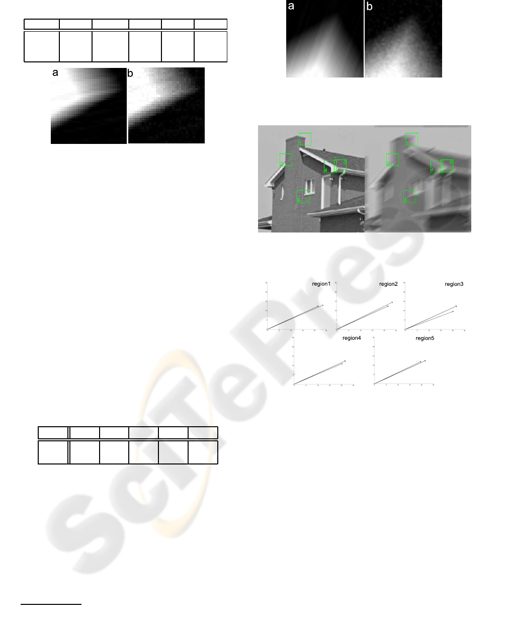
Table 2: Result on synthetic images: v has direction 70 de-
grees and length 30 pixels, σ
η
∈ [0,0.02] and σ
ξ
∈ [0,0.08].
σ
η
| σ
ξ
0 0.02 0.04 0.06 0.08
0 1.95% 1.08% 1.95% 2.23% 0.98%
0.01 3.04% 0.31% 3.99% 1.43% 2.54%
0.02 9.39% 10.11% 6.55% 7.65% 7.50%
Figure 8: Synthetic test images used psf directed 10 degrees
and length 20 pixels, in a σ
η
= 0 and σ
ξ
= 0.08, while in b
σ
η
= 0.02 and σ
ξ
= 0 .
5.2.2 Real Images
We perform two tests on real images
1
; in the first test
we replace y+ ξ with a still camera picture, we blur
it using a convolution with a PSF and we finally add
gaussian white noise η. We take house as the original
image and we manually select five squared windows
of side 30 pixels at some corners. Figure 10 shows
the original and the blurred house image (using psf
with direction 30 degrees and length 25 pixels) and
the analyzed regions. Figure 11 shows two vectors in
pixel coordinates, the estimated ˜v (dashed line) and
the vector having true motion parameters (solid line),
for each selected region. Table 3 shows distance be-
tween the endpoints of the two vectors.
Table 3: Estimation error: distance between ˜v endpoint and
displacement vector, expressed in pixels, on each image re-
gion r.
σ
η
r 1 r 2 r 3 r 4 r 5
0 2.07 2.75 3.19 1.87 2.04
0.01 0,32 6.91 3.52 2.64 4.58
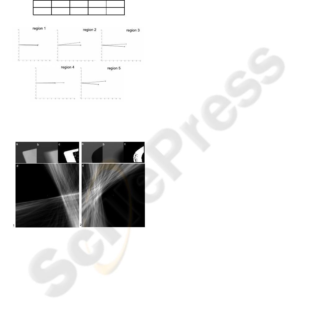
We perform a second experiment using a sequence
of camera images, captured according to the follow-
ing scheme
• a still image, at the initial camera position.
• a blurred image, captured while the camera was
moving.
• a still image, at the final camera position.
We estimated motion blur at some manually selected
corners in the blurred image and we compare results
1
Further images and experimental result are available at
http://www.elet.polimi.it/upload/boracchi
Figure 9: Example of synthetic test images used, psf was
directed 70 degrees and length 30 pixels, in a σ
η
= 0 and
σ
ξ
= 0.08, while in b σ
η
= 0.02 and σ
ξ
= 0 .
Figure 10: Original and blurred house image. Blur have
direction 30 degrees and 25 pixels length, regions analyzed
are numbered.
Figure 11: Displacement vectors ˜v estimated in selected re-
gions of camera images. The solid line is the true displace-
ment vector, while the dotted line represents the estimated
vector ˜v.
with the ground truth, given by matching corner found
by Harris detector in the images taken at the initial and
at the final camera position. Clearly, the accuracy ob-
tained in motion estimation from a single blurred im-
age is lower than that obtained with methods based on
two well focused views. However preliminary results
show good accuracy. For example, motion parameters
estimated in region r 2 are close to the ground truth,
even if the corner is considerably smooth, as it is taken
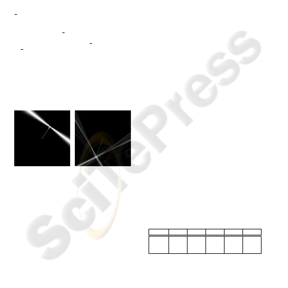
from a common swivel chair. As Figure 13.2 shows,
the votes in parameter space are more spread around
the solution than in Figure 13.1, where the corner is
close to the model of Section 2.2. Table 4 shows re-
sult using the same criteria of Table 3.
Results are less accurate than in previous experiments
because according to experimental settings, motion
PSF could be not perfectly straight or not perfectly
uniform, because of camera movement. This affects
algorithm performances since it approximates motion
blur to a vectorial PSF.
Table 4: Estimation error expressed in pixel unit on each
image region r.
r 1 r 2 r 3 r 4 r 5
0.44 1.90 1.09 3.95 3.75
Figure 12: Displacement vectors ˜v estimated in camera im-
ages. In each plot, the solid line indicates the true displace-
ment vector obtained by matching corners of pictures at ini-
tial and final camera position. Dotted line represents the
estimated displacement vector ˜v.
Figure 13: Figure a Original corner in image b blurred cor-
ner, c set D
0
of considered pixels and d votes in the space
parameter.
6 ONGOING WORK AND
CONCLUDING REMARKS
Results from the experiments, performed both on syn-
thetic and natural images, show that the image at
blurred corners has been suitably modelled and that
the solution proposed is robust enough to cope with
artificial noise and to deal with real images.
However, we noticed that there are only a few useful
corners in real images. This is mostly due to back-
ground and corner non uniformity because of shad-
ows, occlusions or because the original image itself
shows significant intensity variations.
We are actually investigating a procedure to automat-
ically detect blurred corners in a given image and to
adaptively select image regions around them. In this
paper we use squared regions but there are no restric-
tions on their shape, which could be adaptively se-
lected to exclude background elements which would
be considered in D
0
. We believe that estimating blur
on adaptively selected regions could significantly im-
prove the algorithm performance on real images.
We are also investigating an extension of our algo-
rithm to deal with corners which are moving like
Figure 4 b or at least to discern which corners satisfy
our image model.
Finally, we are looking for a criteria to estimate the
goodness of an estimate, as up to now, we consider
the value of the maximum voted parameter pairs.
REFERENCES
Bertero, M. and Boccacci, P. (1998). Introduction to Inverse
Problems in Imaging. Institute of Physics Publishing.
Choi, J. W., Kang, M. G., and Park, K. T. (1998). An al-
gorithm to extract camera-shaking degree and noise
variance in the peak-trace domain.
Harris, C. and Stephens, M. (1988). A combined corner and
edge detector.
Immerkær, J. (1996). Fast noise variance estimation.
Kawamura, S., Kondo, K., Konishi, Y., and Ishigaki, H.
(2002). Estimation of motion using motion blur for
tracking vision system.
Klein, G. and Drummond, T. (2005). A single-frame visual
gyroscope.
Lin, H.-Y. (2005). Vehicle speed detection and identifica-
tion from a single motion blurred image.
Lin, H.-Y. and Chang, C.-H. (2005). Automatic speed mea-
surements of spherical objects using an off-the-shelf
digital camera.
Mikolajczyk, K., Tuytelaars, T., Schmid, C., Zisserman, A.,
Matas, J., Schaffalitzky, F., Kadir, T., and Gool, L. V.
(2005). A comparison of affine region detectors.
Rekleitis, I. (1996). Steerable filters and cepstral analysis
for optical flow calculation from a single blurred im-
age.
Yitzhaky, Y. and Kopeika, N. S. (1996). Identification of
blur parameters from motion-blurred images.
