
COLOR MODELS OF SHADOW DETECTION IN VIDEO SCENES
Csaba Benedek
P
´
azm
´
any P
´
eter Catholic University, Department of Information Technology, Pr
´
ater utca 50/A, Budapest, Hungary
Tam
´
as Szir
´
anyi
Distributed Events Analysis Research Group, Computer and Automation Institute, Kende u. 13-17, Budapest, Hungary
Keywords:
Shadow, color spaces, MRF.
Abstract:
In this paper we address the problem of appropriate modelling of shadows in color images. While previous
works compared the different approaches regarding their model structure, a comparative study of color models
has still missed. This paper attacks a continuous need for defining the appropriate color space for this main
surveillance problem. We introduce a statistical and parametric shadow model-framework, which can work
with different color spaces, and perform a detailed comparision with it. We show experimental results regard-
ing the following questions: (1) What is the gain of using color images instead of grayscale ones? (2) What
is the gain of using uncorrelated spaces instead of the standard RGB? (3) Chrominance (illumination invari-
ant), luminance, or ”mixed” spaces are more effective? (4) In which scenes are the differences significant?
We qualified the metrics both in color based clustering of the individual pixels and in the case of Bayesian
foreground-background-shadow segmentation. Experimental results on real-life videos show that CIE L*u*v*
color space is the most efficient.
1 INTRODUCTION
Detection of foreground objects is a crucial task in vi-
sual surveillance systems. If we can retrieve the accu-
rate silhouettes of the objects, or object groups, their
high-level description becomes much easier, so it is
favorable e.g. in detection of people (Havasi et al.,
2006) or vehicles (Rittscher et al., 2000), respectively
in activity analysis (Stauffer and Grimson, 2000).
The presence of moving shadows on the background
makes difficult to estimate shape or behavior of the
objects, therefore, shadow detection is an important
issue in the applications. However, we do not need
to search for shadows cast on the foreground objects,
since these ’self-shadowed’ scenario parts consist to
the foreground.
We find a thematic overview on several shadow detec-
tors in (Prati et al., 2003). The methods are classified
in groups based on their model structures, and the per-
formance of the different model-groups are compared
via test sequences. The authors note that the methods
work in different color spaces, like RGB (Mikic et al.,
2000) and HSV (Cucchiara et al., 2001), however, it
remains open-ended, how important is the appropri-
ate color space selection, and which color space is
the most effective regarding shadow detection. More-
over, we find also further examples: (Rittscher et al.,
2000) used only gray levels for shadow segmenta-
tion, other approaches were dealing with the CIE
L*u*v* (Martel-Brisson and Zaccarin, 2005), respec-
tively CIE L*a*b* (Rautiainen et al., 2001) spaces.
For the above reasons, the main issue of this paper
is to give an experimental comparison of different
color models regarding cast shadow detection on the
video frames. For the comparison, we propose a gen-
eral model framework, which can work with different
color spaces. During the development of this frame-
work, we have carefully considered the main ap-
proaches in the state-of-the art. Our presented model
is the generalization of our previous work (Benedek
and Szir
´
anyi, 2006).
225
Benedek C. and Szirányi T. (2007).
COLOR MODELS OF SHADOW DETECTION IN VIDEO SCENES.
In Proceedings of the Second International Conference on Computer Vision Theory and Applications - IFP/IA, pages 225-232
Copyright
c
SciTePress

2 BASIC NOTES
In (Prati et al., 2003), the authors distinguished de-
terministic methods (e.g. (Cucchiara et al., 2001)),
which use on/off decision processes at each pixel, and
statistical approaches (see (Mikic et al., 2000)) which
contain probability density functions to describe the
shadow-membership of a give image point. The clas-
sification of the methods whether they are determinis-
tic or statistical depends often only on interpretation,
since deterministic decisions can be done using prob-
abilistic functions also. However, statistical methods
have been widely distributed recently, since they can
be used together with Markov Random Fields (MRF)
to enhance the quality of the segmentation signifi-
cantly (Wang et al., 2006).
First, we developed a deterministic method which
classifies the pixels independently, since that way, we
could perform a relevant quantitative comparison of
the different color spaces. After that we gave a prob-
abilistic interpretation to this model and we inserted
it into a MRF framework which we developed ear-
lier (Benedek and Szir
´
anyi, 2006). We compared the
different results after MRF optimization qualitatively
and observed similar relative performance of the color
spaces to the deterministic model.
Another important point of view regarding the cate-
gorization of the algorithms in (Prati et al., 2003) is
the discrimination of the non parametric and para-
metric cases. Non parametric, or ’shadow invariant’
methods convert the video images into an illuminant
invariant feature space: they remove shadows instead
of detecting them. This task is often performed by a
color space transformation, widely used illumination-
invariant color spaces are e.g. the normalized rgb
(Cavallaro et al., 2004),(Paragios and Ramesh, 2001)
and C
1
C
2
C
3
spaces (Salvador et al., 2004). (We re-
fer later to the normalized rgb as rg space, since
the third color component is determined by the first
and second.) In (Salvador et al., 2004) we find an
overview on these approaches indicating that several
assumptions are needed regarding the reflecting sur-
faces and the lightings. We have found in our experi-
ments that these assumptions are usually not fulfilled
in an outdoor environment, and these methods fail
several times. Moreover, we show later that the rg
and C
1
C
2
C
3
spaces are less effective also in the para-
metric case.
For the above reasons, we developed a parametric
model: we extracted feature vectors from the actual
and mean background values of the pixels and applied
shadow detection as solving a classification problem
in that feature space. This approach is widespread in
the literature, and the key points are the way of feature
extraction, the color space selection and the shadow-
domain description in the feature space. In Section
3, we introduce the feature vector which character-
izes the shadowed pixels effectively. In Section 4,
we describe the chosen shadow domain in the feature
space, and define the deterministic pixel classification
method. We show the quantitative classification re-
sults with the deterministic model regarding five real-
world video sequences in Section 5. Finally, we in-
troduce the MRF framework and analyse the segmen-
tation results in Section 6.
We use three assumptions in the paper: (1) The cam-
era stands in place and has no significant ego-motion.
(2) The background objects are static (e.g. there is no
waving river in the background), ad the topically valid
’background image’ is available in each moment (e.g.
by the method of (Stauffer and Grimson, 2000)). (3)
There is one emissive light source in the scene (the
sun or an artificial source), but we consider the pres-
ence of additional effects (e.g. reflection), which may
change the spectrum of illumination locally.
3 FEATURE VECTOR
Here, we define features for a parametric case where
a shadow model can be constructed including some
challenging environmental conditions. First, we in-
troduce a well-known physical approach on shadow
detection with marking that its model assumptions
may not be fulfilled in real-world video scenes. In-
stead of constructing a more difficult illumination
model, we overcome the appearing artifacts with a
statistical description. Finally, the efficiency of the
proposed model is validated by experiments.
3.1 Physical Approach on Shadow
Detection
According to the illumination model (Forsyth, 1990)
the response g(s) of a given image sensor placed at
pixel s can be written as
g(s) =
e(λ, s)ρ(λ, s)ν(λ)dλ, (1)
where e(λ, s) is the illumination function, ρ(s) de-
pends on the surface albedo and geometric, ν(λ) is
the sensor sensitivity. Accordingly, the difference in
the shadowed and illuminated background values of
a given surface point is caused by the different local
value of e(λ, s) only. For example, outdoors, the il-
lumination function is the composition of the direct
(sun), diffused (sky) and reflected (from other non-
emissive objects) light components in the illuminated

background, while in the shadow the effect of the di-
rect component is missing.
Although the validity of eq. (1) is already limited by
several scene assumptions (Forsyth, 1990), in general,
it is still too difficult to exploit appropriate informa-
tion about the corresponding background-shadow val-
ues, since the components of the illumination func-
tion are unknown. With further strong simplifications
(Forsyth, 1990) eq.(1) implies the well-known ’con-
stant ratio’ rule. Namely, the ratio of the shadowed
g
sh
(s) and illuminated value g
bg
(s) of a given surface
point is considered to be constant over the image:
g
sh
(s)
g
bg
(s)
= A, (2)
where A is the shadow ’darkening factor’, and it does
not depend on s.
In the CCD camera model (Forsyth, 1990) the RGB
sensors are narrow banded and the constant ratio
rule is valid for each color channel independently.
Accordingly, the shadow descriptor is a triple
[A
r
, A
g
, A
b
] containing the ratios of the shadowed
and illuminated background values for the red, green
and blue channels. Due to the deviation of the scene
properties from the model assumptions (Forsyth,
1990), imprecise estimation of the background values
(Stauffer and Grimson, 2000) and further artifacts
caused by video compression and quantification,
the ratio of the shadowed and estimated background
values is never constant. However, to prescribe a
domain instead of a single value for the ratios results
a powerful detector (Siala et al., 2004). In this
way, shadow detection is a one-class-classification
problem in the three dimensional color ratio space.
3.2 Constant Ratio Rule in Different
Color Spaces
In this section, we examine, how can we use the pre-
vious physical approach in different color systems.
We begin the description with some notes. We as-
sume that the video images are originally available
in the RGB color space, and for the different color
space conversions, we use the equations in (Tkalcic
and Tasic, 2003). The ITU D65 standard is used for
calibration of the CIE L*u*v* and L*a*b* spaces. In
the HSV, CIE L*u*v* and L*a*b* spaces we should
discriminate two types of color components. One
component is related to the brightness of the pixel (V,
respectively L*; we refer them later as ’luminance’
components), while the other components correspond
to the ’chrominances’. We classify the color spaces
also: since the normalized rg and C
1
C
2
C
3
spaces con-
tain only chrominance components we will call them
’chrominance spaces’, while grayscale and RGB are
purely ’luminance spaces’. In this terminology, HSV,
CIE L*u*v* and L*a*b* are ’mixed spaces’.
As we stated in the last section, the ratios of the shad-
owed and illuminated values of the R, G, B color
channels regarding a given pixel are near to a global
reference value [A
r
, A
g
, A
b
]. In the following, we
show by experiments that the ’constant ratio rule’ is a
reasonable approximation regarding the ’luminance’
components of other color spaces also.
While shadow may darken the ’luminance’ values of
the pixels significantly the changes in the ’chromi-
nances’ is usually small. In (Cucchiara et al., 2001),
the hue difference was considered as a zero-mean
noise factor. This approach is sometimes inaccurate,
for example outdoors, due to the ambient light of the
blue sky, the shadow shifts to the ’blue’ color domain
(Fig 1, third column). We show that modeling the off-
set between the shadowed and illuminated ’chromi-
nance’ values of the pixels with a Gaussian additive
term is appropriate.
To sum it up, if the current value of a given pixel in a
given color space is [x
0
, x
1
, x
2
] (the indices 0, 1, 2 cor-
respond to the different color components), the esti-
mated background value is there [m
0
, m
1
, m
2
], we de-
fine the shadow descriptor
ψ = [ψ
0
, ψ
1
, ψ
2
] by the fol-
lowing. For i = {0, 1, 2}:
• If i is the index of a ’luminance’ component:
ψ
i
(s) =
x
i
(s)
m
i
(s)
. (3)
• If i is the index of a ’chrominance’ component:
ψ
i
(s) = x
i
(s) −m
i
(s). (4)
We classify s as shadowed point, if its
ψ(s) value lies
in a prescribed domain.
The efficiency of this feature selection can be ob-
served in Fig. 1, where we plot the one dimensional
marginal histograms of the occurring ψ
0
, ψ
1
and
ψ
2
values for manually marked shadowed and fore-
ground points of a 100-frames long outdoor surveil-
lance video sequence (’Entrance pm’). Apart from
some outliers, the shadowed ψ
i
values lie for each
color space and each color component in a ’short’ in-
terval, while the difference of the upper and lower
bounds of the foreground values is usually greater.
However, there is significant overlap between the
one dimensional foreground and shadow histograms,
therefore, as we examine in the next section, an effec-
tive shadow domain description is needed.
We define the descriptor in grayscale and in the rg
space similarly to eq. (3) and (4) considering that
ψ
will be a one, respectively two dimensional vector in
these cases.
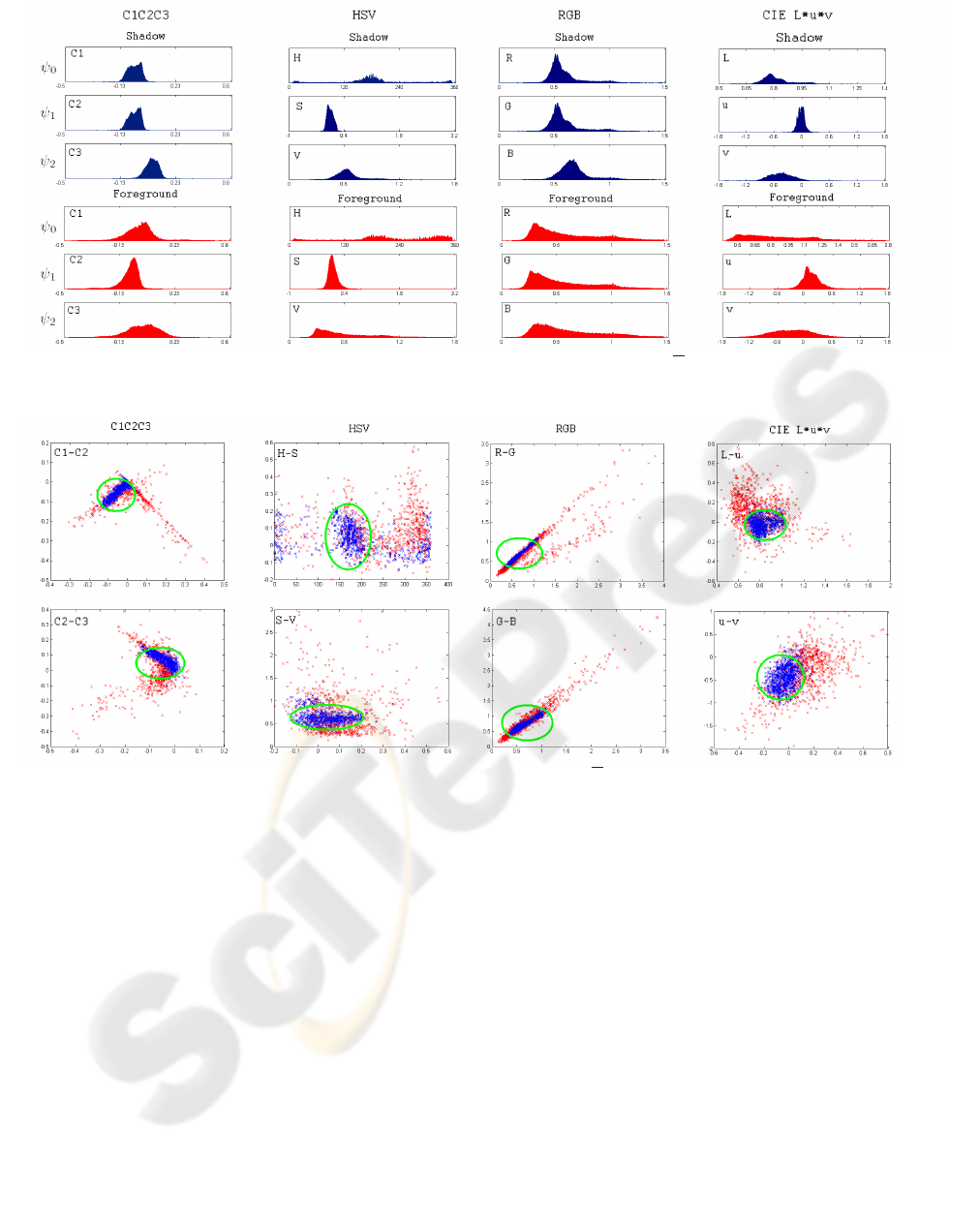
Figure 1: One dimensional projection of histograms of foreground (red) and shadow (blue) ψ values in the ’Entrance pm’ test
sequence.
Figure 2: Two dimensional projection of foreground (red) and shadow (blue) ψ values in the ’Entrance pm’ test sequence.
Green ellipse is the projection of the optimized shadow boundary.
4 SHAPE OF THE SHADOW
DOMAIN
The shadow domain is usually defined by a mani-
fold having a prescribed number of free parameters,
which fit the model to a given scene/situation. Previ-
ous methods used different approaches. The domain
of shadows in the feature space is usually an inter-
val for grayscale images (Wang et al., 2006). Re-
garding color scenes, this domain could be a three
dimensional rectangular bin (Cucchiara et al., 2001):
ratio/difference values for each channel lie between
defined threshold; an ellipsoid (Mikic et al., 2000), or
it may have general shape, like in (Siala et al., 2004).
In the last case a Support Vector Domain Description
is proposed in the RGB color ratios’ space.
By each domain-selection we must consider overlap
between the classes, e.g. there may be foreground
points whose feature values are in the shadow do-
main. Therefore, the chosen shadow-domain should
be not only large enough, containing ’almost all’ the
feature values corresponding to the occurring shad-
owed points, but also ’narrow’ to decrease the num-
ber of the background or foreground points which are
erroneously classified as shadows.
Accordingly, if we ’only’ prescribe that a shadow
descriptor should be accurate, the most general do-
main shape seems to be the most appropriate. How-
ever, in practise, a corresponding problem appears:
the shadow domain may alter significantly (and often
rapidly) in time due to the changes in the illumination
conditions, and adaptive models are needed to follow

these changes. It is sometimes not possible to train
a model with supervision regarding each forthcoming
case of illumination. Therefore, those domains are
preferred, which have less free parameters, and we
can construct an update strategy regarding them.
For these reasons, we used an elliptical shadow do-
main descriptor having parallel axes with the xyz co-
ordinate axes:
Pixel s is shadowed ⇔
2
∑
i=0
ψ
i
(s) −a
i
b
i
2
≤ 1, (5)
where {a
i
, b
i
| i = 0, 1, 2} are the shadow domain pa-
rameters. For these parameters, a similar update pro-
cedure can be constructed to that we introduced in
(Benedek and Szir
´
anyi, 2006). We found in the exper-
iments, that the parameters of the ’chrominance’ com-
ponents are approximately constant in time. Although
the mean darkening ratio of the ’luminance’ compo-
nents may change significantly, it can be estimated
by finding the peak of the joint foreground-shadow ψ
histograms, which can be constructed without super-
vision, with an effective background subtraction algo-
rithm (e.g. (Stauffer and Grimson, 2000)).
We note that with the SVM method (Siala et al.,
2004), the number of free parameters is related to the
number of the support vectors, which can be much
greater than the six scalars of our model. Moreover,
for each situation, a novel SVM should be trained. For
these reasons, we preferred the ellipsoid model, and
in the following we examine its limits. For the sake
of completeness, we note that the domain defined by
eq. (5) becomes an interval if we work with grayscale
images, and a two dimensional ellipse in the rg space.
We visualize the shadow domain of the ’Entrance pm’
test sequence in Fig. 2, where the two dimensional
projection of the occurring foreground and shadow
ψ values are shown corresponding to different color
space selections. We can observe that the components
of vector
ψ are strongly correlated in the RGB space
(and also in C
1
C
2
C
3
), and the previously defined el-
lipse cannot present a narrow boundary. (It would
be better to fit an ellipse with arbitrary axes, but that
choice would cause more free parameters in the sys-
tem.) In the HSV space, the shadowed values are not
within a convex hull, even if we considered that the
hue component is actually periodical (hue = k ∗ 2π
means the same color for each k = 0, 1, . . .). Based
on the above facts, the CIE L*u*v* space seems to
be a good choice. In the next section, we support this
statement by experimental results.
5 COMPARATIVE EVALUATION
WITH THE ELLIPSE MODEL
In this section, we show the tentative limits of the el-
liptical shadow domain defined by eq. (5). The evalu-
ations were done through manually generated ground
truth sequences regrading the following five videos:
• ’Laboratory’ test sequence from the benchmark
set (Prati et al., 2003). This shot contains a simple
indoor environment.
• ’Highway’ video (from the same benchmark set).
This sequence contains dark shadows but ho-
mogenous background without illumination arti-
facts.
• ’Entrance am’, ’Entrance noon’ and ’Entrance
pm’ sequences captured by the ’Entrance’ (out-
door) camera of our university campus in different
parts of the day. These sequences contain difficult
illumination and reflection effects and suffer from
sensor saturation (dark objects and shadows).
The evaluation metrics was the foreground-shadow
discrimination rate. Denote the number of correctly
identified foreground pixels of the evaluation se-
quence by T
F
. Similarly, we introduce T
S
for the num-
ber of well classified shadowed points, A
F
and A
S
is
the number of all the foreground, respectively shad-
owed ground truth points. The discrimination rate is
defined by:
D =
T
F
+ T
S
A
F
+ A
S
. (6)
Since the goal is to compare the limits of the dis-
crimination regarding different color systems, we op-
timized the parameters in eq. (5) through the training
data with respect to maximize the discrimination rate.
We summarized the discrimination rates in Fig. 3,
regarding the test sequences. We can observe that
the CIE L*a*b* and L*u*v* produce the best re-
sults. However, the relative performance of the other
color systems is strongly different in different videos
(see also Table 1). In sequences containing dark
shadows (Entrance pm, highway), the ’chrominance
spaces’ produce poor results, while the gray, RGB and
Lab/Luv results are similarly effective. If shadow is
brighter (Entrance am, Laboratory), the performance
of the ’chrominance spaces’ becomes reasonable, but
the ’luminance spaces’ are relatively poor. (In this
case, shadow is characterized better by the illuminant
invariant features than the luminance darkening do-
main). Since the hue coordinate in HSV is very sensi-
tive to the illumination artifacts (Section 3), the HSV
space is effective only in case of light-shadow.
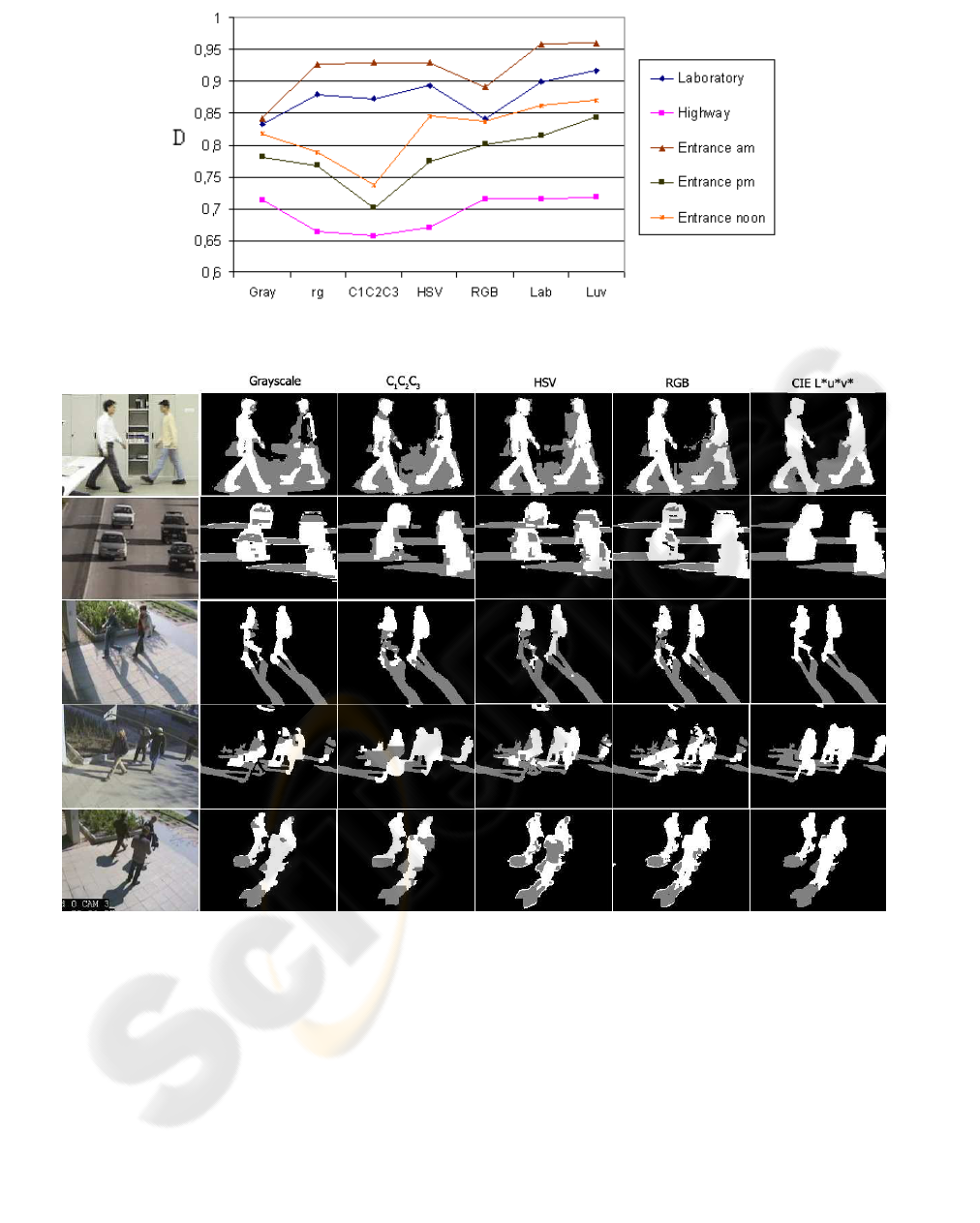
Figure 3: Foreground-shadow discrimination coefficient (D in eq. (6)) regarding different sequences.
Figure 4: MRF segmentation results with different color models. Test sequences (up to down): ’Laboratory’, ’Highway’,
’Entrance am’, ’Entrance pm’, ’Entrance noon’.
6 SEGMENTATION BY USING
BAYESIAN OPTIMIZATION
For practical use, the above color model should be
inserted into a background-foreground-shadow seg-
mentation process. Since we want to test the color
model itself, we use a Markov Random Field (MRF)
optimization procedure (Geman and Geman, 1984) to
get the globally optimal segmentation upon the above
model.
The results in the previous section confirm that using
the defined elliptical shadow domain, the CIE L*u*v*
color space is the most effective to separate shadowed
and foreground pixels only considering their colors,
if we have enough training data. However, in several
applications, we should consider the following facts:
1. Representative ground truth foreground-shadow
points are not available, the optimal ellipse param-

Table 1: Indicating the two most successful and the two less
effective color spaces regarding each test sequence. We also
denote the mean of the darkening factor for shadows in the
third column.
Video Scene Dark Worst Best
Laboratory indoor 0.73 gray,
RGB
Luv,
Lab
Entrance am outdoor 0.50 gray,
RGB
Luv,
Lab
Entrance pm outdoor 0.39 C
1
C
2
C
3
,
rg
Luv,
Lab
Entrance
noon
outdoor 0.35 C
1
C
2
C
3
,
rg
Luv,
Lab
Highway outdoor 0.23 C
1
C
2
C
3
,
rg
Luv,
RGB
eters should be estimated somehow.
2. The classification of a given pixel is usually done
considering not only its color, but also the class of
the neighbors (MRF).
Here we suit the proposed model to an adaptive
Bayesian model-framework, and show that the advan-
tage of using the appropriate color space can be mea-
sured directly in the applications.
The segmentation framework is a Markov Random
Field (Geman and Geman, 1984), more specifically
a Potts model (Potts, 1952). An image S is consid-
ered to be a two-dimensional grid of pixels (sites),
with a neighborhood system on the lattice. The pro-
cedure assigns a label ω
s
to each pixel s ∈ S form the
label-set: L = {bg,sh,fg} corresponding to the three
classes: foreground (fg), background (bg) and shadow
(sh). Therefore, the segmentation is equivalent with
a global labeling Ω = {ω
s
| s ∈ S}. Each class at
each pixel position is characterized by a conditional
density function: p
k
(s) = P(x
s
|ω
s
= k), k ∈ L, s ∈ S.
Eg. p
bg
(s) is the probability of the fact that the back-
ground process generates the observed color value x
s
at pixel s.
Following the Potts model, the optimal segmentation
corresponds to the labeling which minimizes:
b
Ω = argmin
Ω
∑
s∈S
−p
ω
s
(s) +
∑
r,q∈S
Φ(ω
r
, ω
q
), (7)
where the Φ term is responsible for getting
smooth, connected regions in the segmented image.
Φ(ω
r
, ω
q
) = 0 if q and r are not neighboring pixels,
otherwise:
Φ(ω
r
, ω
q
) =
−β if ω
r
= ω
q
+β if ω
r
6= ω
q
The definition of the density functions p
bg
(s) and
p
fg
(s) s ∈ S is the same, as we defined in (Benedek
and Szir
´
anyi, 2006). We use a mixture of Gaus-
sian model for the pixel values in the background,
where the parameters are determined using (Stauf-
fer and Grimson, 2000). The foreground probabilities
come from spatial pixel value statistics (Benedek and
Szir
´
anyi, 2006).
Before inserting our model in the previously defined
MRF framework, we give to the shadow-classification
step defined in Section 4 a probabilistic interpretation.
We rewrite eq. (5): we match the current
ψ(s) value
of pixel s to a probability density function f (
ψ(s)),
and decide its class:
pixel s is shadowed ⇔ f (ψ(s)) ≥ t. (8)
The domains defined by eq. (5) and eq. (8) are equiv-
alent, if f is a Gaussian density function (η):
f (
ψ(s)) = η(ψ(s), µ
ψ
, Σ
ψ
) =
=
1
(2π)
3
2
q
detΣ
ψ
exp
−
1
2
(
ψ(s) − µ
ψ
)
T
Σ
−1
ψ
(ψ(s) − µ
ψ
)
with the following parameters: µ
ψ
= [a
0
, a
1
, a
2
]
T
,
Σ
ψ
= diag{b
2
0
, b
2
1
, b
2
2
}, while t = (2πb
0
b
1
b
2
)
−
3
2
e
−
1
2
.
Using Gaussian distribution for the occurring fea-
ture values is supported also by the one dimensional
marginal histograms in Fig. 1.
In the following, the way of using the previously de-
fined probability density functions in the MRF model
is straightforward: p
sh
(s) = f (
ψ(s)). The flexibil-
ity of this MRF model comes from the fact that we
defined ψ(s) shadow descriptors for different color
spaces differently in Section 3. The method sets the
parameters of the class models adaptively, similarly to
(Benedek and Szir
´
anyi, 2006). Using a desktop com-
puter, and the ICM MRF-optimization technique, the
algorithm runs with 3fps on 320×240 video frames.
We compared the segmentation results using differ-
ent color spaces in the MRF model (Fig. 4), and ob-
served that the quality of the segmentation depends
on the used color space similarly to that we measured
in Section 5 .
7 CONCLUSION
This paper examined the color modeling problem of
shadow detection. We developed a model framework
for this task, which can work with different color
spaces. Meanwhile, the model can detect shadows un-
der significantly different scene conditions and it has
a few free parameters which is advantageous in prac-
tical point of view. In our case, the transition between
the background and shadow domains is described by

statistical distributions. With this model, we com-
pared several well known color spaces, and observed
that the appropriate color space selection is an impor-
tant issue regarding the segmentation results. We val-
idated our method on five video shots, including well-
known benchmark videos and real-life surveillance
sequences, indoor and outdoor shots, which contain
both dark and light shadows. Experimental results
show that CIE L*u*v* color space is the most effi-
cient both in the color based clustering of the indi-
vidual pixels and in the case of Bayesian foreground-
background-shadow segmentation.
REFERENCES
Benedek, C. and Szir
´
anyi, T. (2006). Markovian framework
for foreground-background-shadow separation of real
world video scenes. In Proc. Asian Conference on
Computer Vision. LNCS, 3851.
Cavallaro, A., Salvador, E., and Ebrahimi, T. (2004). De-
tecting shadows in image sequences. In Proc. of IEEE
Conference on Visual Media Production.
Cucchiara, R., Grana, C., Neri, G., Piccardi, M., and Prati,
A. (2001). The sakbot system for moving object de-
tection and tracking. In Video-Based Surveillance
Systems-Computer Vision and Distributed Processing.
Forsyth, D. A. (1990). A novel algorithm for color con-
stancy. In International Journal of Computer Vision.
Geman, S. and Geman, D. (1984). Stochastic relaxation,
gibbs distributions and the bayesian restoration of im-
ages. IEEE Trans. Pattern Analysis and Machine In-
telligence, pages 721–741.
Havasi, L., Szl
´
avik, Z., and Szir
´
anyi, T. (2006). Higher or-
der symmetry for non- linear classification of human
walk detection. Pattern Recognition Letters, 27:822 –
829.
Martel-Brisson, N. and Zaccarin, A. (2005). Moving cast
shadow detection from a gaussian mixture shadow
model. In IEEE Computer Society Conference on
Computer Vision and Pattern Recognition.
Mikic, I., Cosman, P., Kogut, G., and Trivedi, M. M. (2000).
Moving shadow and object detection in traffic scenes.
In Proceedings of International Conference on Pattern
Recognition.
Paragios, N. and Ramesh, V. (2001). A mrf-based real-time
approach for subway monitoring. In Proc. IEEE Con-
ference in Computer Vision and Pattern Recognition.
Potts, R. (1952). Some generalized order-disorder transfor-
mation. In Proceedings of the Cambridge Philosoph-
ical Society.
Prati, A., Mikic, I., Trivedi, M. M., and Cucchiara, R.
(2003). Detecting moving shadows: algorithms and
evaluation. IEEE Trans. Pattern Analysis and Ma-
chine Intelligence, (7):918–923.
Rautiainen, M., Ojala, T., and Kauniskangas, H. (2001).
Detecting perceptual color changes from sequential
images for scene surveillance. IEICE Transactions on
Information and Systems, pages 1676 – 1683.
Rittscher, J., Kato, J., Joga, S., and Blake, A. (2000). A
probabilistic background model for tracking. In Proc.
European Conf. on Computer Vision.
Salvador, E., Cavallaro, A., and Ebrahimi, T. (2004). Cast
shadow segmentation using invariant color features.
Comput. Vis. Image Underst., (2):238–259.
Siala, K., Chakchouk, M., Chaieb, F., and O.Besbes (2004).
Moving shadow detection with support vector domain
description in the color ratios space. In Proceedings of
the 17th International Conference on Pattern Recog-
nition.
Stauffer, C. and Grimson, W. E. L. (2000). Learning
patterns of activity using real-time tracking. IEEE
Trans. Pattern Analysis and Machine Intelligence,
22(8):747–757.
Tkalcic, M. and Tasic, J. (2003). Colour spaces - percep-
tual, historical and applicational background. In Proc.
Eurocon 2003.
Wang, Y., Loe, K.-F., and Wu, J.-K. (2006). A dynamic
conditional random field model for foreground and
shadow segmentation. IEEE Trans. Pattern Analysis
and Machine Intelligence, 28(2):279–289.
