DETECTION OF PERFECT AND APPROXIMATE REFLECTIVE
SYMMETRY IN ARBITRARY DIMENSION
Darko Dimitrov and Klaus Kriegel
Freie Universit
¨
at Berlin, Institute of Computer Science
Takustrasse 9, D-14195 Berlin, Germany
Keywords:
Reflective Symmetry, Geometric Hashing, Principal Component Analysis.
Abstract:
Symmetry detection is an important problem with many applications in pattern recognition, computer vision
and computational geometry. In this paper, we propose a novel algorithm for computing a hyperplane of re-
flexive symmetry of a point set in arbitrary dimension with approximate symmetry. The algorithm is based on
the geometric hashing technique. In addition, we consider a relation between the perfect reflective symmetry
and the principal components of shapes, a relation that was already a base of few heuristic approaches that
tackle the symmetry problem in 2D and 3D. From mechanics, it is known that, if H is a plane of reflective
symmetry of the 3D rigid body, then a principal component of the body is orthogonal to H. Here we extend
that result to any point set (continuous or discrete) in arbitrary dimension.
1 INTRODUCTION AND
RELATED WORK
Symmetry is one of the most important features of
shapes and objects, which is proved to be a power-
ful concept in solving problems in many areas includ-
ing detection, recognition, classification, reconstruc-
tion and matching of different geometrics shapes, as
well as compression of their representations. In gen-
eral, symmetry in Euclidean space can be defined in
terms of three transformations: translation, rotation
and reflection. A subset P of R
d
is approximately
symmetric with respect to transformation T if for a
big enough subset P
′
of P, the distance between T(P
′
)
and P
′
is less then small constant ε, where the distance
is measured using some appropriate metric, for exam-
ple Hausdorff, RMS (root mean square) or bottleneck
distance measures as most commonly used metrics.
If P
′
= P and ε = 0, then T(P) = P, and we say that
P is perfectly symmetric with respect to T. In this
paper we are interested in both approximate and per-
fect symmetry in terms of transformation of reflection
through a hyperplane.
In what follows, we briefly survey the most rel-
evant existing algorithms and techniques, we are
aware of, for identifying both perfect and approxi-
mate symmetry.
Traditional approaches consider perfect symme-
try in discrete settings as a global feature. Some of
these methods reduced the symmetry detection prob-
lem to a detection of symmetries in circular strings
(Atallah, 1985; Wolter et al., 1985; Highnam, 1986;
Zhang and Huebner, 2002), for which efficient so-
lutions are known (Knuth et al., 1977). Other effi-
cient algorithms based on the octree representation
(Minovic et al., 1993), the extended Gaussian im-
age (Sun and Sherrah, 1997) or the singular value
decomposition of the points of the model (Shah and
Sorensen, 2005) also have been proposed. Further,
methods for describing local symmetries were devel-
oped. (Blum, 1967) proposed an algorithm based on
a medial axis transform. An algorithm presented in
(Thrun and Wegbreit, 2005) detects perfect symme-
tries in range images, exploiting taxonomy of differ-
ent types of symmetries and relations between them,
by explicitly searching an increasing sets of points.
A very recent approach, based on generalized mo-
ment functions and their spherical harmonics repre-
sentation, was introduced by (Martinet et al., 2006).
However, since the above mentioned methods con-
sider only perfect symmetries, they may be inaccu-
rate in detection the symmetry for shapes with added
128
Dimitrov D. and Kriegel K. (2007).
DETECTION OF PERFECT AND APPROXIMATE REFLECTIVE SYMMETRY IN ARBITRARY DIMENSION.
In Proceedings of the Second International Conference on Computer Vision Theory and Applications - IU/MTSV, pages 128-136
Copyright
c
 SciTePress

noise or missing data.
As a result to this challenge, several algorithms
for measuring imperfect symmetries have been de-
veloped. For example, Zabrodsky et al. proposed
an algorithm based on a measure of symmetry, de-
fined as minimum mean squared distance required to
transform a shape into a symmetric shape (Zabrodsky
et al., 1993; Zabrodsky et al., 1995). A method of
detecting a line of approximate symmetry of 2D im-
ages considering only the boundary of the image, us-
ing a hierarchy of certain directional codes, was pre-
sented in (Parui and Majumder, 1983). Marola in-
troduced a measure of reflective symmetry with re-
spect to a given axis where global reflective symmetry
is found by roughly estimating the axis location and
then fine tuning the location by minimizing the sym-
metry measure (Marola, 1989). Kazhdan et al. intro-
duced the symmetry descriptors, a collection of spher-
ical functions that describe the measure of a model
symmetry with respect to every axis passing through
the center of gravity (Kazhdan et al., 2003; Kazhdan
et al., 2004). Very recently, Podolak et al. proposed
the planar reflective symmetry transform, which mea-
sures the symmetry of an object with respect to all
planes passing through its bounding volume (Podolak
et al., 2006). A method of detecting planes of reflec-
tive symmetry, by exploiting the topological config-
uration of the edges of a 2D sketch of a 3D objects,
was developed by (Zou and Lee, 2005). Mitra et al.
proposed a method of finding partial and approximate
symmetry in 3D objects (Mitra et al., 2006). Their ap-
proach relies on matching geometry signatures (based
on the concept of normal cycles) that are used to ac-
cumulate evidence for symmetries in an appropriate
transformation space.
Till now, most of the research was dedicated to
investigation of symmetry in 2D and 3D. Here, we
consider two approaches which lead to algorithms in
arbitrary dimension. The contribution of this work is
two-fold. First, we propose a novel algorithm, based
on geometric hashing, for computing the reflectional
symmetry of point sets with approximate symmetry in
arbitrary dimension. Second, we give a proof of the
relation between the perfect reflective symmetry and
the principal components of discrete or continuous
geometrical objects in arbitrary dimensions. The rela-
tion, in the case when rigid objects in 3D are consid-
ered, is known from mechanics and is established by
analyzing a moment of inertia (Symon, 1971). With-
out rigorous proof for other cases than 3D rigid ob-
jects, this result was a base as a heuristic in several
symmetry detection algorithms (Minovic et al., 1993;
O’Mara and Owens, 1996; Sun and Sherrah, 1997).
Banerjee et al. also tackle this relation in 3D, in the
case when the objects are represented as 3D binary
arrays, but a formal proof is missing in their paper
(Banerjee et al., 1994).
The rest of the paper is organized as follows: In
Section 2 we present the algorithm based on geomet-
ric hashing for computing a reflectional symmetry of
a point set with approximate symmetry. The behavior
of the algorithm in the 2D case is estimated by prob-
abilistic analysis and evaluated on real and synthetic
data. In Section 3, we give a proof of the relation be-
tween the perfect reflective symmetry and the princi-
pal components of geometrical objects in arbitrary di-
mensions. Conclusions and indications of future work
are given in Section 4.
2 DETECTION OF REFLECTIVE
SYMMETRY: GEOMETRIC
HASHING APPROACH
Geometric hashing is a recognition technique based
on matching of transformation-invariant object repre-
sentations stored in a hash table (Wolfson and Rigout-
sos, 1997; Alt and Guibas, 1999). Here, we assume
that the given point set P ⊆ R
d
is approximately sym-
metric, and our goal is to compute the hyperplane of
symmetry H
sym
with a geometric hashing technique.
More precisely, hashing is utilized to compute the
normal vector of H
sym
. Additionally, one could use
the fact that the center of gravity of P lies on H
sym
in
the case when P has a perfect symmetry, or with high
probability near to H
sym
in the case when P is approx-
imately symmetric. However, to be on the safe side,
if some outliers cause that the center of gravity is far
from H
sym
, we can apply a second phase of geometric
hashing to compute a point on H
sym
.
We start from the hypothesis that each point pair
(p,q) is a candidate for a pair of points that are sym-
metric with respect to H
sym
. Without loss of gener-
ality, we assume that the first coordinate of p is less
than or equal to the first coordinate of q. If p is sym-
metric to q, the vector
−→
pq is orthogonal to H
sym
. We
note that this vector is characterized uniquely by the
tuple of angles (α
2
,α
3
,...,α
d
) where α
i
is the angle
between
−→
pq and the i-th vector of the standard base of
R
d
.
Since we assume at least a weak form of sym-
metry, we can expect that the number of point pairs
(approximately) symmetric regarding H
sym
, is bigger
than the number of point pairs (approximately) sym-
metric regarding any other hyperplane H. For exam-
ple, if we have a perfect symmetric point set with n
points, then we have
n
2
point pairs perfectly symmet-

ric regarding H
sym
. In contrast to that, the hyperplanes
corresponding to remaining

n
2

−
n
2
point pairs are
randomly distributed. See Fig. 1 for illustration in
R
2
.
S
1
’
S
2
S
2
’
CS
1
α
α
Figure 1: The angle α between y-axis and the line seg-
ments s
1
s
′
1
and s
2
s
′
2
, formed by symmetric points, occurs
two times. All other angles occurs only once.
In the standard approach of geometric hashing
a number K ∈ N is fixed and the interval [0,π] is
subdivided into K subintervals of equal length π/K.
Then, the hash function maps a tuple of angles
(α
2
,α
3
,...,α
d
) to a tuple of integers (a
2
,a
3
,...,a
d
),
where each a
i
denotes the index of the subinterval
containing α
i
, i.e.,
a
i
=

α
i
· K
π

.
Equivalently one can describe this approach with
a so-called voting scheme by subdividing the cube
[0,π]
d−1
into a grid with K
d−1
cells. Each cell is
equipped with a counter, collecting votes of all point
pairs whichs angle tuple is contained in the cell. In the
end one has to search for the cell with the maximum
number of votes. However, this simple idea has some
drawbacks related to the choice of K. Since K
d−1
is a
lower bound for both, time and storage complexity of
the algorithm, K should not be too large. Moreover,
if K is large, the noise might cause that the peak of
votes is distributed over a larger cluster of cells. On
the other side, if K is small, the preciseness of the re-
sult is not satisfactory.
We overcome these problems generalizing an idea
from (Pleißner et al., 1999) that combines a rather
coarse grid structure with a quite precise information
about the normal vector. To this end, we use coun-
ters for the grid’s vertices instead of counters for the
grid’s cells. Any vote (α
2
,α
3
,...,α
d
) for a grid cell
(a
2
,...,a
d
) will be distributed to the incident vertices
of the cell such that vertices close to (α
2
,α
3
,...,α
d
)
get a larger portion of the vote than more distant ver-
tices.
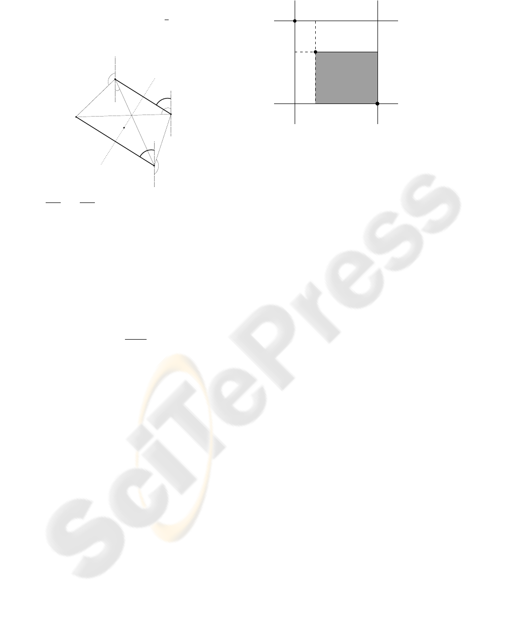
v
v by the shaded area
increasing the score of
v
opp
α
Figure 2: Updating the score for the angle vector α =
(α
1
,α
2
).
To explain this idea more precisely, we introduce
some more notations. Let Q be a grid cell, and v a grid
vertex incident with Q. Among the vertices incident
with Q, there is exactly one, called the opposite ver-
tex v
opp
, that differs in all d − 1 coordinates from v.
If
~
α = (α
2
,α
3
,··· ,α
d
) is a vote for Q (i.e., a point in
Q) we denote by Q(
~
α,v) the (axis-parallel) subcube
of Q spanned by the points
~
α and v. It is clear that the
closer
~
α is to v the larger is the volume of Q(
~
α,v
opp
).
Thus, the unit score of
~
α will be distributed to all
vertices incident with Q such that each vertex v gets
the score vol(Q(
~
α),v
opp
)/vol(Q). See Figure 2 for
illustration in R
3
. We remark that K
d−1
counters suf-
fice for (K + 1)
d−1
grid vertices because the scoring
scheme must be treated as cyclic structure in the sense
that any vertex of the form (β
2
,...,π,...,β
d
) is iden-
tified with (π− β
2
,...,0,...,π − β
d
).
Outline of the algorithm.
Input: A set of n points P ∈ R
d
,d ≥ 2, with approxi-
mate symmetry.
Output: An approximation of H
sym
.
1. Let X be the set of all point pairs (p,q) from P
such that the first coordinate of p is less than or
equal to the first coordinate of q. Compute for
each pair the angle tuple
~
α = (α
2
,...,α
d
).
2. Install a voting scheme of K
d−1
counters and set
all counters to 0.
3. For each (p,q) ∈ X with
~
α = (α
2
,...,α
d
) deter-
mine the corresponding grid cell Q. For all ver-
tices v incident with Q, add to the counter of v the
vote vol(Q(
~
α),v
opp
)/vol(Q).
4. Search for the vertex v = v
max
with the largest
score w. Compute the angle tuple of the approxi-
mate normal vector of H
sym
as the weighted center
of gravity of v and its neighboring vertices with

the following formula:
~
β =
wv+
∑
d
i=2
w
+
i
v
+
i
+
∑
d
i=2
w
−
i
v
−
i
w+
∑
d
i=2
w
+
i
+
∑
d
i=2
w
−
i
,
where v
+
i
,v
−
i
,2 ≤ i ≤ d, denote the neighbor-
ing vertices of v, and w
+
i
,w
−
i
their corresponding
scores. Let~n be a normal vector in R
d
correspond-
ing to the angle tuple
~
β.
5. Approximate a point on H
sym
selecting all pairs
(p,q) ∈ X that vote for v
max
(i.e.,
~
α is in a cell in-
cident with v
max
). For each selected pair project
the center c = (p + q)/2 onto the line spanned
by the normal vector ~n and store the position of
the projected point on that line in a 1-dimensional
scoring scheme. Use the maximal score to extrap-
olate the location of a point on H
sym
analogously
as in 4.
Taking into account that we can keep the parameter
K small, the crucial step of the algorithm is the third
one, because it requires the processing of Θ(n
2
) point
pairs. However, it is possible to reduce this effort un-
der the assumption that the center of gravity c(P) is
close to H
sym
. This holds whenever the points without
symmetric counterpart are distributed regularly in the
sense that their center of gravity is close to the center
of gravity of the symmetric point set. In this case it
is sufficient to consider votes of pairs (p, q) of points
with nearly equal distances to c(P). If δ is a bound for
both, the distance of c(P) to H
sym
and the distortion
of the symmetric counterpart of a point with respect
to H
sym
, the first step of the algorithm can be replaced
as follows:
• Compute the center of gravity c(P).
• Order the points of P with respect to the distance
to c(P).
• For all points q ∈ P find the first point p
i
and the last point p
j
in the ordered list
such that dist(p
i
,c(P)) ≥ dist(q,c(P)) − 2δ and
dist(p
j
,c(P)) ≤ dist(q, c(P)) + 2δ and form X
from the pairs {q, p
k
}, i ≤ k ≤ j.
Although this modification does not improve the run
time in the worst case, it effects a remarkable speed
up of the algorithm for real world data.
2.1 Probabilistic Analysis and Evaluation
of the Algorithm in 2D Case
The 2D version of the algorithm has been imple-
mented and tested on real and synthetic data. The
generation of the synthetic data is based on a prob-
abilistic model, which additionally can be used for
λ
λ
B
+
B
−
p
−
p
+
p
−
ǫ
α
∼
Figure 3: Point set generation.
a probabilistic analysis of the reliability of the algo-
rithm.
The model incorporates the following two aspects
of an approximately symmetric point set P. First, for
the majority of the points p ∈ P there is a counter-
part
e
p that is located close to the symmetric position
of p, where the symmetry, with out loss of generality,
is defined with respect to the x-axis. Second, there
is a smaller subset of points in P without symmetric
counterpart. To obtain such a point set, we apply the
following procedure (see Fig. 3 for illustration). In
the upper half of the unit ball B
+
, we uniformly gen-
erate a random point set P
+
with n points. In the lower
half B
−
we reflect the point set P
+
over the x-axis and
perturb it randomly. So, we obtain the set of points
e
P
−
= {(x± δ
x
,−y± δ
y
) | (x,y) ∈ P
+
}, where (δ
x
, δ
y
)
is random point from the ball B((0, 0),ε). Addition-
ally, we generate a random point set M in B, with
m points, which do not have symmetric counterpart.
Point set M represents an additional noise in the form
of missing/extra points in the input data set.
Most pairs of symmetric points span a line that
is nearly parallel to the y-axis. A vote of such pair
will be called a good vote. Nevertheless, for points
p
+
∈ P
+
that are close to the x-axis the perturbation
of p
−
might cause a bigger angle α between the y-
axis and the line spanned by
f
p
−
and p
+
. A vote from
such point pairs, as well as votes from nonsymmetric
point pairs, will be called bad. Thus, we introduce a
parameter λ > 0 defining a stripe of width 2λ along
the x-axis such that all symmetric point pairs without
this stripe have good votes.
Our goal is to derive an upper bound for ε that
makes almost sure, that the given symmetry line cor-
responds to a maximal peak in the scoring scheme.
We first estimate the width of the interval collecting
the votes of the majority of the correct point pairs re-
garding to the symmetry line. On the other side, we
will show that the probability, that another interval of
the the same width would collect the same order of

Table 1: Empirical probability of finding correct line of reflective symmetry for different values of the ”noise” parameters ε
and k.
k \ ε 0.01 0.005 0.004 0.003 0.002 0.001 0.0
0.9 0.90 0.92 0.93 0.94 0.94 0.95 0.95
0.8 0.91 0.93 0.94 0.95 0.95 0.96 0.96
0.7 0.91 0.93 0.94 0.94 0.95 0.96 0.97
0.6 0.94 0.93 0.96 0.96 0.97 0.99 0.99
0.5 0.96 0.99 0.96 0.99 1.0 1.0 1.0
0.4 1.0 1.0 1.0 1.0 1.0 1.0 1.0
0.3 1.0 1.0 1.0 1.0 1.0 1.0 1.0
0.2 1.0 1.0 1.0 1.0 1.0 1.0 1.0
0.1 1.0 1.0 1.0 1.0 1.0 1.0 1.0
0.0 1.0 1.0 1.0 1.0 1.0 1.0 1.0
votes, is very small for bounded ε.
Since the scoring scheme is a cyclic structure, it
also makes sense to speak about negative angles: es-
pecially, angles α ∈ (
π
2
,π) will be identified with the
negative angles α− π ∈ (−
π
2
,0). According to Fig. 3,
for a symmetric point pair outside the λ stripe we have
the following bound on the angle α which defines the
vote of the pair: sinα ≤
ε
2λ
, or |α| ≤ arcsin
ε
2λ
. Since
arcsin
ε
h
≤
π
2
ε
h
≤
π
2
ε
2λ
, we have
|α| ≤ arcsin
ε
2λ
≤
πε
4λ
. (1)
We set γ(ε,λ) :=
πε
4λ
and introduce for any angle β the
random variable V
β
counting all votes of the random
point set P that fall into the interval [β − γ(ε,λ),β +
γ(ε,λ)].
Let A
1
= π/2 denote the area of the upper half
of the unit ball and A
2
= 2λ denote the area of
the rectangle over the horizontal diameter of the
unit ball with height λ. Thus, the probability that
a point p ∈ P
+
generates a good pair is at least
q =
A
1
−A
2
A
1
= (1−
4λ
π
). Since V
0
is at least the sum S
of n independent variables
X
i
=

1 with probability q;
0 with probability 1− q,
we have
E(V
0
) ≥ E(S) = nq, (2)
and
Pr[V
0
< t] ≤ Pr[S < t],t > 0. (3)
Combining (3) with the Chernoff inequality
Pr[S < E[S] −t] ≤ e
−2t
2
/n
, for t = E[S]/2 = nq/2,
we obtain the following estimation:
Pr(V
0
< nq/2) ≤ e
−q
2
n/2
. (4)
Let N ≤

2n+m
2

be the number of points pairs with bad
votes, and consider an angle β, where |β| > 2γ(ε,λ),
i.e., X
β
doesn’t count any good vote. The expectation
of X
β
is
E(X
β
) = N
2γ(ε,λ)
π
= N
ε
2λ
. (5)
Applying the Markov inequality Pr[X
β
> t] ≤
E(X
β
)
t
,
for t = nq/2, we obtain
Pr[X
β
> nq/2] ≤
N ε
λqn
. (6)
We would like to note that in the case of X
β
, we can-
not apply any of the Chernoff’s inequalities, which in
general give better bounds than the Markov inequal-
ity, because X
β
is not a sum of independent random
variables.
Now, we come to the ultimate goal of this analysis
- to estimate Pr[V
β
> V
0
] and to study when it is small,
i.e., when the algorithm gives a correct answer with
high probability. From
Pr[V
β
> V
0
] ≤ Pr[V
β
> t] + Pr[V
0
< t],t > 0, (7)
(4) and (6), we obtain
Pr[V
β
> V
0
] ≤ e
−q
2
n/2
+
N ε
λπq
. (8)
The first term of the right side of (8) is signifi-
cantly smaller then the second term. This can be ex-
plained by the fact that the first term was obtained by
the Chernoff inequality, and the second term by the
weaker Markov inequality. However, for ε = o(
1
n
) the
second term will be also small, and then the algorithm
will work well with high probability.
As described above, we randomly generated 100
point sets with same parameters ε and k, where k is
the ratio between the number of additional points and
the number of good point pairs (k = m/n). Table 1
shows the empirical probability of finding the correct
angle of the symmetry line. We present here only

those combination of ε and k for which the empiri-
cal probability was at least 0.9. The results indicate
that the algorithms is less sensitive to noise, due to
missing/extra data, then to noise that comes from im-
perfect symmetry of the points. This conclusion is
consistent with the theoretical analysis we have ob-
tained. Namely, ε and N occur at the same place in
the last term of the relation (8). The number of addi-
tional points m occurs in the relation (8) through N.
The other variable which determines N is n, and its
contribution to the value of N is bigger than that of m.
Therefore, m has smaller influence to the expression
than ε.
We tested the algorithm also on real data sets. The
tests were performed on pore patterns of copepods - a
group of small crustaceans found in the sea and nearly
every freshwater habitat (see Fig. 4). The pores in a
pattern were detected as points by the method based
on a combination of hierarchical watershed transfor-
mation and feature extraction methods presented in
(Pleißner et al., 1999). The algorithm successfully de-
tected the symmetry line because the extracted point
sets have relatively good reflective symmetry, and ma-
jority of the points (around 90%) have a symmetric
counterpart.
3 DETECTION OF REFLECTIVE
SYMMETRY: PCA APPROACH
Another approach for an efficient detection of the
hyperplane of perfect reflective symmetry in arbi-
trary dimension is that based on principal component
analysis (Jolliffe, 2002). To the best of our knowl-
edge, this approach was used as heuristic without rig-
orous proof (also confirmed in communication with
other researchers in this area (O’Mara and Owens,
2005)). A relation between the principal components
and symmetry of an object, in the case of rigid ob-
jects in 3D, was establish in mechanics by analyzing
a moment of inertia (Symon, 1971). This result, in
the context of detecting the symmetry, was first ex-
ploit by (Minovic et al., 1993). Here we extend that
result to any set of points (continuous or discrete) in
arbitrary dimension. The central idea and motivation
of PCA (also known as the Karhunen-Loeve trans-
form, or the Hotelling transform) is to reduce the di-
mensionality of a data set by identifying the most sig-
nificant directions (principal components). Let P =
{p
1
, p
2
,..., p
m
}, where p
i
is a d-dimensional vector,
and c = (c
1
,c
2
,...,c
d
) ∈ R
d
be the center of gravity
of P. For 1 ≤ k ≤ d, we use p
ik
to denote the k-th
coordinate of the vector p
i
. Given two vectors u and
v, we use hu,vi to denote their inner product. For any
Figure 4: Left side: illustrations of different types of cope-
pods. Right side: a pore pattern of a copepod.
unit vector v ∈ R
d
, the variance of P in direction v is
var(P,v) =
1
m
m
∑
i=1
hp
i
− c,vi
2
. (9)
The most significant direction corresponds to the unit
vector v
1
such that var(P, v
1
) is maximum. In gen-
eral, after identifying the j most significant directions
B
j
= {v
1
,v
2
,...,v
j
}, the ( j + 1)-th most significant
direction corresponds to the unit vector v
j+1
such that
var(P,v
j+1
) is maximum among all unit vectors per-
pendicular to v
1
,v
2
,...,v
j
.
It can be verified that for any unit vector v ∈ R
d
,
var(P,v) = hCv,vi, (10)
whereC is the covariance matrix of P. C is a symmet-
ric d × d matrix where the ij-th component, C
ij
,1 ≤
i, j ≤ d, is defined as
C
ij
=
1
m
m
∑
k=1
(p
ik
− c
i
)(p
jk
− c
j
). (11)
The procedure of finding the most significant di-
rections, in the sense mentioned above, can be formu-
lated as an eigenvalue problem. If λ
1
> λ
2
> · · · > λ
d
are the eigenvalues of C, then the unit eigenvector v
j
for λ
j
is the j-th most significant direction. All λ
j
s
are non-negative and λ
j
= var(P,v
j
). Since the ma-
trix C is symmetric positive definite, its eigenvectors
are orthogonal. If the eigenvalues are not distinct, the
eigenvectors are not unique. In this case, an orthog-
onal basis of eigenvectors is chosen arbitrary. How-
ever, we can achieve distinct eigenvalues by a slight
perturbation of the point set.
In the case when P is a continuous set of d-
dimensional vectors, all above expressions have anal-
ogons defined in terms of integrals instead of finite
sums. Due to the space limitation, we omit them here.
Now, we prove the following connection between
hyperplane reflective symmetry and principal compo-
nents.

Theorem 3.1 Let P be a d-dimensional point set
symmetric with respect to a hyperplane H
sym
and as-
sume that the covariance matrix C has d different
eigenvalues. Then, a principal component of P is or-
thogonal to H
sym
.
Proof. Without loss of generality, we can assume that
the hyperplane of symmetry is spanned by the last d −
1 standard base vectors of the d-dimensional space
and the center of gravity of the point set coincides
with the origin of the d-dimensional space, i.e., c =
(0,0,...,0). Then, the components C
1j
and C
j1
are 0
for 2 ≤ j ≤ d, and the covariance matrix has the form:
C =




C
11
0 ... 0
0 C
22
... C
2d
.
.
.
.
.
.
.
.
.
.
.
.
0 C
d2
... C
dd




(12)
Its characteristic polynomial is
det(C− λ I) = (C
11
− λ) f(λ), (13)
where f(λ) is a polynomial of degree d − 1, with co-
efficients determined by the elements of the (d − 1) ×
(d − 1) submatrix of C. From this it follows that C
11
is a solution of the characteristic equation, i.e., it is an
eigenvalue of C and the vector (1, 0, ...,0) is its cor-
responding eigenvector (principal component), which
is orthogonal to the assumed hyperplane of symmetry.

As an immediate consequence of Theorem 3.1 we
have:
Corollary 3.2 Let P be a perfectly symmetric point
set in arbitrary dimension. Then, any hyperplane of
reflective symmetry is spanned by n-1 principal axes
of P.
The corollary implies a straightforward algorithm for
finding the hyperplane of reflective symmetry of a
point set in arbitrary dimension.
Outline of the algorithm.
Input: A set of n points P ∈ R
d
,d ≥ 2, with approxi-
mate symmetry.
Output: An approximation of H
sym
.
1. Compute the covariance matrix C of P.
2. Compute the eigenvectors of C and the candidate
hyperplanes of reflective symmetry.
3. Reflect the points through every candidate hyper-
plane.
4. Find if each reflected point is enough close to a
point in P. The correspondence between reflected
points and points in P is bijection.
The first and third step of the algorithm have linear
time complexity in the number of points. Computa-
tion of the eigenvectors, when d is not very large, can
be done in O(d
3
) time, for example with Jacobi or QR
method (Press et al., 1995). Computing the candidate
hyperplanes can be done in O(d). Therefore, for fixed
d, the time complexity of the second step is constant.
For very large d, the problem of computing eigenval-
ues is non-trivial. In practice, the above mentioned
methods for computing eigenvalues converge rapidly.
In theory, it is unclear how to bound the running time
combinatorially and how to compute the eigenvalues
in decreasing order. In (Cheng et al., 2005) a mod-
ification of the Power method (Parlett, 1998) is pre-
sented, which can give a guaranteed approximation
of the eigenvalues with high probability. However,
for reasonable big d the most expensive step is the
forth one. Here we can apply an algorithm for nearest
neighbor search, for example the algorithm based on
Voronoi diagram, which together with preprocessing
has run time complexity O(nlogn), d = 2, or O(n
⌈
d
2
⌉
),
d ≥ 3. If we consider point sets with perfect symme-
try, then in the 4-th step, it suffices to check if the
reflection of a point of P is identical with other point
of P. For this, we will need to sort the points lexi-
cographically, and since this is computationally most
expensive part in the whole algorithm, it follows that
the above algorithm in the case of detecting perfect
symmetry has time complexity O(nlogn) in arbitrary
dimension.
In what follows, we discuss two problems that
may arise in theory, but are relatively uncommon in
practice. The first one considers the case when the
eigenvalues are not distinct, and the other the case
when one or more variables are zero.
Equality of eigenvalues, and hence equality of
variances of PCs, will occur for certain patterned ma-
trices. The effect of this occurrence is that for a group
of q equal eigenvalues, the corresponding q eigen-
vectors span a certain unique q-dimensional space,
but, within this space, they are, apart from being or-
thogonal to one another, arbitrary. In the context of
our problem, it means that the d-dimensional point
set will have exactly d candidates as hyperplanes of
symmetry only when the eigenvalues of the covari-
ance matrix are distinct. For example, if we have 3-
dimensional point set, then if exactly 2 eigenvalues
of the covariance matrix are equal, than the point set
might has rotational and reflective symmetry. If the
all 3 are equal, the point set might have any type of
symmetry, including spherical symmetry. To justify
this geometrically, we can imagine what happens to
the covariance ellipsoid in this cases. For example,
in the case when all 3 eigenvalues are equal it be-

comes a ball. In the case when the eigenvalues are
not distinct, we can slightly perturb the point set, and
obtain unique approximate hyperplanes of reflective
symmetry.
The case when q variances equal zero, implies
that the rank of covariance matrix of the point set
diminishes for q. Therefore we can reduce the d-
dimensional problem to a (d − q)-dimensional prob-
lem.
Beside its simplicity and efficiency, as it is known,
detecting symmetry by PCA has two drawbacks. PCA
fails to identify potential hyperplanes of symmetry,
when the eigenvalues of the covariance matrix of the
object are not distinct. The second drawback is that
PCA approach cannot guaranty the correct identifica-
tion when the symmetry of the shape is too weak.
4 CONCLUSION AND FUTURE
WORK
The most of the research effort on symmetry detection
was dedicated to shapes and object in 2D and 3D. In
this paper, we proposed a novel algorithm which is
also able to detect a hyperplane of reflective symme-
try in arbitrary dimension. The algorithm is based on
the modified version of geometric hashing. We have
implemented a 2D variant of the algorithm. The be-
havior of the algorithm was analyzed with a proba-
bilistic model. The tests on real and synthetic data
showed that the algorithm is robust when the symme-
try is not too weak, and that it is quite insensitive on
outlayers.
The second contribution of this paper is the proof
of the relation between the reflective symmetry and
principal components of any type of symmetric ge-
ometric shapes in arbitrary dimension. The only re-
lated result to this is the result known from the me-
chanics, which establish the above relation for rigid
bodies in 3D. We present here a stronger result, which
confirms this relation for any symmetric geometric
shape in arbitrary dimension. That opens a possibility
to generalize some already known ideas from 2D and
3D in higher dimensions.
An implementation of the geometric hashing al-
gorithm in higher dimensions and estimations of its
behavior is one of the tasks for future work. Of
course, the 3D case is of the biggest practical impor-
tance. Comparing the results obtained by both here
presented algorithms, as well as comparing them with
other algorithms for detecting reflective symmetry is
of interest.
REFERENCES
Alt, H. and Guibas, L. (1999). Discrete geometric shapes:
Matching, interpolation, and approximation. In Sack,
J.-R. and Urrutia, J., editors, Handbook of Computa-
tional Geometry, pages 121 – 153. Elsevier Science
Publishers B.V. North-Holland, Amsterdam.
Atallah, M. J. (1985). On symmetry detection. In IEEE
Trans. on Computers c-34, 7, pages 663–666.
Banerjee, D. K., Parui, S. K., and Majumder, D. D. (1994).
Plane of symmetry of 3d objects. In Proc. of the 29th
Annual Convention of the Computer Society of India.
Information Technology for Growth and Prosperity.,
pages 39–44.
Blum, H. (1967). A transformation for extracting new de-
scriptors of shape. In Models for the Perception of
Speech and Visual Form, pages 362–380. MIT Press,
W. Whaten-Dunn, Ed.
Cheng, S.-W., Wang, Y., and Wu, Z. (2005). Provable di-
mension detection using principal component analy-
sis. In Proc. of the 21st ACM Symposium on Compu-
tational Geometry, pages 208–217.
Highnam, P. T. (1986). Optimal algorithms for finding the
symmetries of a planar point set. Inf. Process. Lett.,
22(5):219–222.
Jolliffe, I. T. (2002). Principal Component Analysis.
Springer, 2nd edition.
Kazhdan, M., Chazelle, B., Dobkin, D., Funkhouser, T., and
Rusinkiewicz, S. (2003). A reflective symmetry de-
scriptor for 3d models. Algorithmica, 38, pages 201 –
225.
Kazhdan, M., Funkhouser, T., and Rusinkiewicz, S. (2004).
Symmetry descriptors and 3D shape matching. In
Symposium on Geometry Processing, pages 115–123.
Knuth, D., Morris, J. H., and Pratt, V. (1977). Fast pattern
matching in strings. SIAM Journal of Computing 6, 2,
pages 323–350.
Marola, G. (1989). On the detection of the axes of symme-
try of symmetric and almost symmetric planar images.
IEEE Transactions o Pattern Analysis and Machine
Intelligence, 11(1):104–8.
Martinet, A., Soler, C., Holzschuch, N., and Sillion, F.
(2006). Accurate detection of symmetries in 3d
shapes. ACM Transactions on Graphics, 25(2):439
– 464.
Minovic, P., Ishikawa, S., and Kato, K. (1993). Symmetry
identification of a 3-d object represented by octree. In
IEEE Transaction on Pattern Analysis and Machine
Intelligence, volume 15(5), pages 507–514.
Mitra, N. J., Guibas, L., and Pauly, M. (2006). Partial
and approximate symmetry detection for 3d geome-
try. In ACM Transactions on Graphics, volume 25,
pages 560–568.
O’Mara, D. and Owens, R. (1996). Measuring bilateral
symmetry in digital images. In IEEE TENCON Digi-
tal Signal Processing Application, pages 151–156.
O’Mara, D. and Owens, R. (2005). Private communication.

Parlett, B. N. (1998). The Symmetric Eigenvalue Problem.
SIAM, Philadelphia,PA.
Parui, S. and Majumder, D. (1983). Symmetry analysis by
computer. In Pattern Recognition, volume 16, pages
63–67.
Pleißner, K.-P., Hoffmann, F., Kriegel, K., Wenk, C., Weg-
ner, S., Sahlstr
¨
ohm, A., Oswald, H., Alt, H., and
Fleck, E. (1999). New algorithmic approaches to
protein spot detection and pattern matching in two-
dimensional electrophoresis gel databases. Elec-
trophoresis, 20:755–765.
Podolak, J., Shilane, P., Golovinskiy, A., Rusinkiewicz, S.,
and Funkhouser, T. (2006). A planar-reflective sym-
metry transform for 3D shapes. ACM Transactions on
Graphics (Proc. SIGGRAPH), 25(3):549–559.
Press, W. H., Teukolsky, S. A., Veterling, W. T., and Flan-
nery, B. P. (1995). Numerical Recipes in C: The art
of scientific computing. Cambridge University Press,
New York, USA, second edition.
Shah, M. I. and Sorensen, D. C. (2005). A symmetry pre-
serving singular value decomposition. In SIAM Jour-
nal of Matrix Analysis and it‘s Applications (Octo-
ber).
Sun, C. and Sherrah, J. (1997). 3d symmetry detection using
the extended gaussian image. In IEEE PAMI 19, 2,
pages 164–168.
Symon, K. R. (1971). Mechanics. Reading, MA: Adison-
Wesley, 3rd edition.
Thrun, S. and Wegbreit, B. (2005). Shape from symmetry.
In Proc. International Conference on Computer Vision
(ICCV), pages 1824–1831. IEEE Computer Scoiety.
Wolfson, H. and Rigoutsos, I. (1997). Geometric hashing:
An overview. 24:10–21.
Wolter, J. D., Woo, T. C., and Volz, R. A. (1985). Optimal
algorithms for symmetry detection in two and three
dimensions. The Visual Computer 1, pages 37–48.
Zabrodsky, H., Peleg, S., and Avnir, D. (1993). Completion
of occluded shapes using symmetry. In Proc. CVPR,
pages 678–679.
Zabrodsky, H., Peleg, S., and Avnir, D. (1995). Symmetry
as a continuous feature. Trans. PAMI 17, 12:1154–
1166.
Zhang, J. and Huebner, K. (2002). Using symmetry as a
feature in panoramic images for mobile robot applica-
tions. In Proc.Robotik, volume 1679 of VDI-Berichte,
pages 263–268.
Zou, H. L. and Lee, Y. T. (2005). Skewed mirror sym-
metry detection from a 2d sketch of a 3d model. In
GRAPHITE ’05: Proc. of the 3rd international con-
ference on Computer graphics and interactive tech-
niques in Australasia and South East Asia, pages 69–
76. ACM Press.