ADAPTIVE DATA-DRIVEN REGULARIZATION FOR
VARIATIONAL IMAGE RESTORATION IN THE BV SPACE
Hongwei Zheng and Olaf Hellwich
Computer Vision & Remote Sensing, Berlin University of Technology
Franklinstrasse 28/29, Sekretariat FR 3-1, D-10587 Berlin
Keywords:
Bayesian estimation, regularization, convex optimization, functions of bounded variation, linear growth func-
tional, self-adjusting, parameter estimation, data-driven, hyperbolic conservation laws, image restoration.
Abstract:
We present a novel variational regularization in the space of functions of Bounded Variation (BV) for adaptive
data-driven image restoration. The discontinuities are important features in image processing. The BV space
is well adapted for the measure of gradient and discontinuities. More over, the degradation of images includes
not only random noises but also multiplicative, spatial degradations, i.e., blur. To achieve simultaneous im-
age deblurring and denoising, a variable exponent linear growth functional on the BV space is extended in
Bayesian estimation with respect to deblurring and denoising. The selection of regularization parameters is
self-adjusting based on spatially local variances. Simultaneously, the linear and non-linear smoothing oper-
ators are continuously changed following the strength of discontinuities. The time of stopping the process
is optimally determined by measuring the signal-to-noise ratio. The algorithm is robust in that it can handle
images that are formed with different types of noises and blur. Numerical experiments show that the algorithm
achieves more encouraging perceptual image restoration results.
1 INTRODUCTION
The primary goal of image restoration is to recover
lost information from a degraded image and obtain
the best estimate to the original image. Its applica-
tions include photography, remote sensing, medical
imaging, and multimedia processing. According to
the image degradation model g = hf + η, given an
observed image function g ∈ L
2
(Ω), with Ω ⊂ R
2
is
an open bounded domain, the problem is to estimate
the original image f with unknown noise η and point
spread function h. In order to solve this ill-posed in-
verse problem, one of the well-known techniques is
by energy minimization and regularization.
In classical Sobolev spaces, we can not make de-
tailed analysis and reasonable measure of discontinu-
ities. A simple image including a white disk on a
black background is not in any Sobolev space, but be-
longs to the BV space. The BV space is the space
of functions for which the sum of the perimeters of
the level sets is finite. Therefore, the BV space is
well adapted for determining discontinuities across or
along edges. Compared to wavelet based methods in
the frequency domain (Gousseau and Morel, 2001),
the assumption of the functions on the BV space is
still too restrictive to represent tiny detailed textures
and infinite discontinuities (Alvarez and Gousseau,
1999). However, currently, the BV space is still a
much larger space than the Sobolev space for mod-
eling images in the spatial domain.
Since the seminal work of the ROF model (Rudin
et al., 1992), the BV space based functionals have
been widely applied to image restoration, super-
resolution approaches, segmentation and related early
vision tasks, e.g., Mumford-Shah functional (Mum-
ford and Shah, 1989), modeling of oscillatory com-
ponents (Meyer, 2001), modeling of inpainting and
super-resolution approaches, (Chan and Shen, 2006).
Recently, (Aubert and Vese, 1997), (Vese, 2001)
propose a convex linear growth functional in the
BV space for deblurring and denoising using Γ-
convergence approximation. (Chen et al., 2006),
(Chen and Rao, 2003) suggest a more general variable
exponent, linear growth functional in the BV space
53
Zheng H. and Hellwich O. (2007).
ADAPTIVE DATA-DRIVEN REGULARIZATION FOR VARIATIONAL IMAGE RESTORATION IN THE BV SPACE.
In Proceedings of the Second International Conference on Computer Vision Theory and Applications - IFP/IA, pages 53-60
Copyright
c
 SciTePress

for image denoising. However, through the literature
study, we find that only little work is done on how
to determine regularization parameters, and diffusion
operators for achieving optimal and high-fidelity im-
age restoration results.
In this paper, we extend the variable exponent,
linear growth functional (Chen et al., 2006), (Chen
and Rao, 2003) to double regularized Bayesian es-
timation for simultaneously deblurring and denois-
ing. The Bayesian framework provides a structured
way to include prior knowledge concerning the quan-
tities to be estimated (Freeman and Pasztor, 2000).
Different from traditional “passive” edge-preserving
methods (Geman and Reynolds, 1992), our method
is an “active” data-driven approach which integrates
self-adjusting regularization parameters and dynamic
computed gradient prior for self-adjusting the fidelity
term and multiple image diffusion operators. A new
scheme is designed to select the regularization pa-
rameters adaptively on different levels based on the
measurements of local variances. The chosen diffu-
sion operators are automatically adjusted following
the strengths of edge gradient. The suggested ap-
proach has several important effects: firstly, it shows
a theoretically and experimentally sound way of how
local diffusion operators are changed automatically
in the BV space. Secondly, the self-adjusting regu-
larization parameters also control the diffusion oper-
ators simultaneously for image restoration. Finally,
this process is relatively simple and can be easily ex-
tended for other regularization or energy optimiza-
tion approaches. The experimental results show that
the method yields encouraging results under different
kinds and amounts of noise and degradation.
The paper is organized as follows. In section 2, we
discuss the concepts of BV space, the total variation
(TV) model and its related functionals. In section 3,
we present a Bayesian estimation based adaptive vari-
ational regularization with respect to the estimation
of PSFs and images. Numerical approximation and
experimental results are shown in section 4. Conclu-
sions are summarized in section 5.
2 RELATED WORK
2.1 The Bv Space and the Tv Method
Following the total variation (TV) functional (Rudin
et al., 1992), (Chambolle and Lions, 1997), (Weickert
and Schn
¨
orr, 2001), (Chan et al., 2002), (Aubert and
Vese, 1997), we study the total variation functional in
the bounded total variation (BV) space.
Definition 2.1.1 BV(Ω) is the subspace of functions
f ∈ L
1
(Ω) where the quantity is finite,
TV( f) =
Ω
|Df|dA = (1)
sup

Ω
f · divϕdA ; ϕ ∈ C
1
c
(Ω,R
N
)

where dA = dxdy, |ϕ(A)|
L
∞
(Ω)
≤ 1, C
1
c
(Ω,R
N
) is
the space of functions in C
1
(Ω) with compact sup-
port Ω. BV(Ω) endowed with the norm k fk
BV(Ω)
=
k fk
L
1
(Ω)
+ TV( f) which is a Banach space.
While one adopts the TV measure for image regular-
ization, the posterior energy for Tikhonov Regulariza-
tion then takes the form which is also given in (Rudin
et al., 1992),
J ( f) =
λ
2
Ω
|
g− hf
|
2
dA+
Ω
|
Df
|
dA (2)
where g is the noisy image, f is an ideal image and
λ > 0 is a scaling regularization parameter. When an
image f is discontinuous, the gradient of f has to be
understood as a measure. The TV( f) functional is
often denoted by
Ω
|Df|dxdy, with the symbol D re-
ferring to the conventional differentiation ∇. One use
f ∈ L
1
(Ω) to simplify the numerical computation (see
(Giusti, 1984), for instance),
Ω
|Df|dA =
Ω
|∇f|dA.
In order to study more precisely the influence of
the smoothing term in the regularization, we need to
make an insight observation of a more general total
variation functional which can help us to understand
the convexity criteria in variational regularization. A
general bounded total variational functional can be
written in the following,
J ( f
(g,h)
) =
λ
2
Ω
(g− hf)
2
dA+
Ω
φ(|∇f(x, y)|)dA
The choice of the function φ is crucial. It determines
the smoothness of the resulting function f in the space
V = { f ∈ L
2
(Ω);∇f ∈ L
1
(Ω)} which is not reflexive.
In this variational energy function, the closeness
of the solution to the data is imposed by the penalty
term φ(·) in the energy function. If the energy func-
tions are nonconvex, it might become more compli-
cated than the convex functionals. Although some
non-convex φ(·) penalty terms can achieve edge-
preserving results, convex penalty terms can help us
to get a global convergence and decrease the complex-
ity of computation. In the following, we study φ(·) in
a more general form φ(∇f) → φ(Df) in the BV space.
2.2 Convex Linear-Growth Functional
Let Ω be an open, bounded, and connected subset
of R
N
. We use standard notations for the Sobolev

W
1,p
(Ω) and Lebesgue spaces L
p
(Ω). A variational
function can be written in the form,
J ( f
(g,h)
) =
λ
2
Ω
(g− hf)
2
dA+
Ω
φ(Df(x, y))dA
where the function
Ω
φ(Df)dA is finite on the space
W
1,1
which is a nonreflexive Banach space.
We recall the notation of lower semicontinuity of
functionals defined on the BV(Ω) space. We denote
by
L
N
the Lebesgue N-dimensional measure R
N
and
by
H
α
the α-dimensional Hausdorff measure. We
say that f ∈ L
1
(Ω) is a function of bounded varia-
tion ( f ∈ BV(Ω)) if its distributed derivative Df =
(D
1
f, ...,D
N
f) belongs to the weakest topology on
M (Ω). M (Ω) is the set of all signed measures on
Ω with bounded total variation.
For any function f ∈ L
1
(Ω), we denote by S
f
the
complement of the Lebesgue set of f . The set S
f
is
of zero Lebesgue measure and is also called the jump
set of f. If f ∈ BV(Ω), then f is differentiable al-
most everywhere on Ω\ S
f
. Moreover, the Hausdorff
dimension of S
f
is at most (N − 1) and for
H
N−1
,
x ∈ S
f
it is possible to find unique f
+
(x), f
−
(x) ∈ R,
with f
+
(x) > f
−
(x) and ν ∈ S
N−1
of unit sphere in
R
N
, such that
lim
r→0
+
r
−N
B
ν
r
(x)
| f(y) − f
+
(y)|dy
= lim
r→0
+
r
−N
B
ν
r
(x)
| f(y) − f
−
(y)|dy = 0 (3)
where B
ν
r
(x) = {y ∈ B
r
(x)} : (y − x) · ν > 0 and
B
−ν
r
(x) = {y ∈ B
r
(x)} : (y − x) · ν < 0. The normal
ν means that they points toward the larger value in
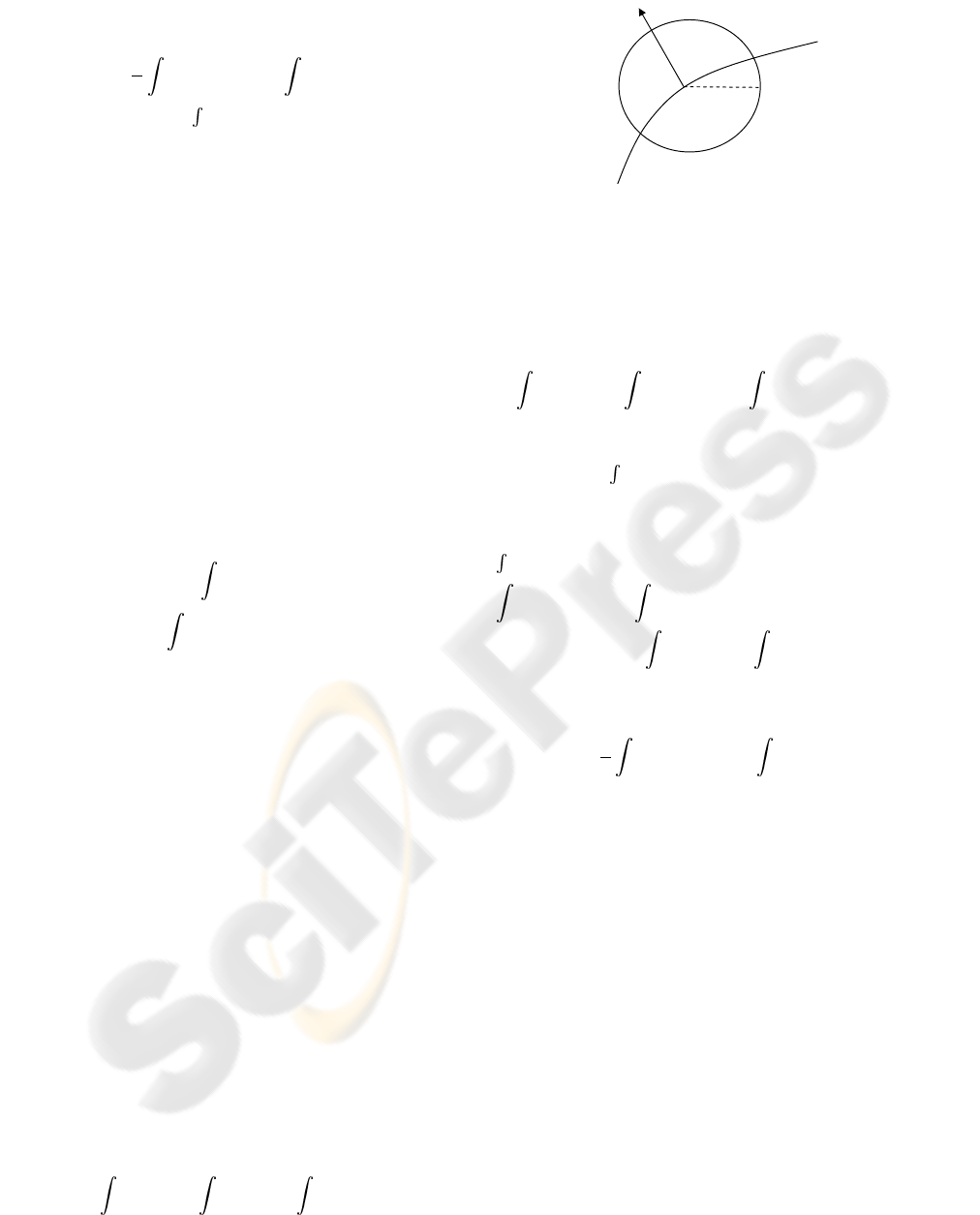
the image f. We denote by B
r
(x) the ball centered in
x of radius r, shown in Fig. 1.
We have the Lebesgue decomposition,
Df = ∇f ·
L
N
+ D
s
f (4)
where ∇f ∈ (L
1
(Ω))
N
is the Radon-Nikodym deriva-
tive of Df with respect to
L
N
. In other words, ∇ f
is the density of the absolutely continuous part of
Df with respect to the Lebesgue measure. We also
have the decomposition for D
s
f = C
f
+ J
f
, where
J
f
= ( f
+
− f
−
)N
f
·
H
N−1
S
is Hausdorff part or jump
part and C
f
is the Cantor part of Df. The measure
C
f
is singular with respect to L
N
and it is diffuse, that
is, C
f
(S) = 0 for every set S of Hausdorff dimension
N − 1.
H
N−1
|S
f
is called the perimeter of related edges
in Ω. Finally, we can write Df and its total variation
on Ω, |Df|(Ω), in the following,
Df = ∇f · L
N
+C
f
+ ( f
+
− f
−
)ν·
H
N−1
|S
f
|Df| =
Ω
|∇f|dx+
Ω\S
f
|C
f
| +
S
f
( f
+
− f
−
)d
H
N−1
|S
f
( )
f
n x
f
S
( )
r
B
x
x
( )x

f
( )x

f
Figure 1: Definition of f
+
, f
−
, and the jump set S
f
.
It is then possible to define the convex function of
measure φ(| · |) on
M (Ω), which is for Df,
φ(|Df|) = φ(|∇ f|) · L
N
+ φ
∞
(1)|D
s
f|, (5)
and the functional following (Goffman and Serrin,
1964),
Ω
φ(|Df|) =
Ω
φ(|∇f|)dx+
Ω
φ
∞
(1)|D
s
f|, (6)
where the functional φ(| · |)(Ω) is proved in weak
topology and lower semi-continuous on
M (Ω). That
is to say that
Ω
φ(|Df|) is convex on BV(Ω), φ is
convex and increasing on R
+
.
By the decomposition of D
s
f, the properties ofC
f
,
J
f
, and the definition of the constant c, the functional
Ω
φ(|Df|) can be written as,
Ω
φ(|Df|) =
Ω
φ(|∇f|)dx
+ c
Ω\S
f
|C
f
| + c
S
f
( f
+
− f
−
)d
H
N−1
|S
f
Based on this equation, the energy functional on the
BV space becomes,
inf
f∈BV(Ω)
J =
λ
2
Ω
(g− hf)
2
dA+
Ω
φ(|Df|)dA (7)
Although some characterization of the solution is pos-
sible in the distributional sense, it remains difficult
to handle numerically. To circumvent the problem,
(Vese, 2001) approximates the BV solution using the
notion of Γ-convergence which is also an approxi-
mation for the well-known Mumford-Shah functional
(Mumford and Shah, 1989). The Mumford-Shah
functional is a sibling of this functional (Chan and
Shen, 2006).
The target of studying these functionals on the BV
space is to understand a more general variable expo-
nent, L
p
linear growth functional which is a deduction
functional on the BV space.
2.3 Variable Exponent Linear-Growth
Functional
While the penalty function is φ(|Df|) → φ(x,|Df |), it
becomes a variable exponent linear growth functional

in the BV space (Chen et al., 2006), (Chen and Rao,
2003),
J ( f
(g,h)
) =
λ
2
Ω
(g− hf)
2
dA+
Ω
φ(x,Df(x,y))dA
For the definition of a convex function of measures,
we refer to the works of (Goffman and Serrin, 1964),
(Demengel and Teman, 1984). According to their
work, for f ∈ BV(Ω), we have,
Ω
φ(x,Df)dA =
Ω
φ(x,∇f)dA+
Ω
|D
s
f|dA (8)
where
φ(x,∇f)dA =
(
1
q(x)
|∇f|
q(x)
, |∇f| < β
|∇f| −
βq(x)−β
q(x)
q(x)
, |∇f| ≥ β
where β > 0 is fixed, and 1 ≤ q(x) ≤ 2. The term
q(x) is chosen as q(x) = 1 +
1
1+k|∇G
σ
∗I(x)|
2
based on
the edge gradients. I(x) is the observed image g(x),
G
σ
(x) =
1
σ
exp[−|x|
2
/(2σ
2
)] is a Gaussian filter. k >
0, σ > 0 are fixed parameters. The main benefit of
this equation is that the local image information are
computed as prior information for guiding image dif-
fusion. This functional including two equations are
both convex and semi-continuous. This leads to a
mathematically sound model for ensuring the global
convergence. This equation is extended in a Bayesian
estimation based double variational regularization not
only for image denoising but also for image deblur-
ring.
3 BAYESIAN ESTIMATION
BASED VARIATIONAL IMAGE
RESTORATION
Following a Bayesian paradigm, the ideal image f,
the PSF h and an observed image g fulfill
P( f,h|g) =
p(g| f,h)P( f,h)
p(g)
∝ p(g| f,h)P( f,h) (9)
Based on this form, our goal is to find the op-
timal estimated image f and the optimal blur
kernel h that maximizes the posterior p( f,h|g).
J ( f|h,g) = −log{p(g| f,h)P( f)} and J (h| f,g) =
−log{p(g| f, h)P(h)} express that the energy cost
J
is equivalent to the negative log-likelihood of the data.
The resulting method attempts to minimize dou-
ble cost functions subject to constraints such as non-
negativity conditions of the image and energy preser-
vation of PSFs. The objective of the convergence is to
minimize double cost functions by combing the en-
ergy function for the estimation of PSFs and images.
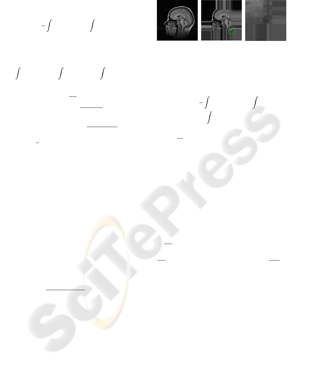
(a) (b) (c)
Figure 2: Homogeneous Neumann Boundary Conditions.
(a) An original MRI head image. (b)(c) Homogeneous
Neumann boundary condition is implemented by mirroring
boundary pixels.
We propose a Bayesian based functional on the BV
spaces. It is formulated according to
J
ε
( f,h) =
λ
2
Ω
(g− hf)
2
dA+ β
Ω
(∇h)dA
+γ
Ω
φ
ε
(x,Df)dA (10)
The Neumann boundary condition (shown in
Fig. 2)
∂f
∂N
(x,t) = 0 on ∂Ω × [0, T] and the initial
conditionf(x, 0) = f
0
(x) = g in Ω are used, where N
is the direction perpendicular to the boundary.
3.1 Alternating Minimization
To avoid the scale problem between the minimization
of PSF and image via steepest descent, an AM method
following the idea of coordinate descent is applied
(Zheng and Hellwich, 2006). The AM algorithm de-
creases complexity.
The equations derived from Eq. (10) are using fi-
nite differences which approximate the flow of the
Euler-Lagrange equation associated with it,
∂
J
ε
∂f
= λ
1
h(−x,−y) ∗ (h∗ f − g) − γdiv(φ(x,∇f))
∂
J
ε
∂h
= λ
2
f(−x,−y)∗ ( f ∗ h− g) − β∇h· div

∇h
|∇h|

Neumann boundary conditions are assumed (Acar
and Vogel, 1994). In the alternate minimization,
blur identification including deconvolution, and data-
driven image restoration including denoising are pro-
cessed alternatingly via the estimation of images and
PSFs. The partially recovered PSF is the prior for the
next iterative image restoration and vice versa. The
algorithm is described in the following:
Initialization:
g(x) = g(x), h
0
(x) is random numbers
while
nmse > threshold
(1). nth
it. f
n
(x) = argmin( f
n
|h
n−1
,g),
fix h
n−1
(x), f(x) > 0
(2). (n+ 1)th
it. h
n+1
= argmin(h
n+1
| f
n
,g),
fix f
n
(x), h(x) > 0
end

While h = I and I is the identity matrix, the al-
ternating minimization of PSFs and images becomes
the estimation of images, e.g., it is corresponding to a
denoising problem. While h 6= I (h is generally a con-
volution operator), it corresponds to a deblurring and
denoising problem. The existence and uniqueness of
solution remain true, if h satisfies the following hy-
potheses: (a) h is a continuous and linear operator
on L
2
(Ω). (b) h does not annihilate constant func-
tions. (c) h is injective. Thereby, we need to consider
the blur kernels at the first step. Further more, we do
deconvolution for the blurred noisy image. Then the
deconvolved image is smoothed by a family of lin-
ear and nonlinear diffusion operators in an alternating
minimization.
3.2 Self-Adjusting Regularization
Parameters
We have classified the regularization parameters λ in
three different levels. Here, we present the method for
the selection of window-based regularization param-
eters λ
w
(window w based λ
w
, the 1st level). When
the size of windows is amplified to the size of an in-
put image, λ becomes a scale regularization param-
eter for the whole image (the 2nd level). If we fix
λ for the whole process, then the selection of regu-
larization parameter is conducted on the level of one
fixed λ for the whole process (the 3nd level). We as-
sume that the noise is approximated by additive white
Gaussian noise with standard deviation σ to construct
a window-based local variance estimation. Then we
focus on the adjustment of parameter λ and operators
in the smoothing term φ. These two computed compo-
nents can be prior knowledge for preserving disconti-
nuities and detailed textures during image restoration.
The Eq. 10 can be formulated in the following,
argmin
Ω
φ(x,Df(x,y))dA subject to
Ω
(g− hf)
2
dA
where the noise is a Gaussian distributed with vari-
ance σ
2
. λ can be a Lagrange multiplier in the fol-
lowing form,
λ =
1
σ
2
|Ω|
Ω
div[φ(x, Df(x,y))] (g− hf)dA (11)
λ is a regularization parameter controlling the “bal-
ance” between the fidelity term and the penalty term.
The underlying assumption of this functional satisfies
k fk
BV(Ω)
= k fk
L
1
(Ω)
+ TV( f) in the BV space. The
distributed derivative |D f| generates an approxima-
tion of input “cartoon model”and oscillation model
(Meyer, 2001). Therefore, this process preserves
discontinuities during the elimination of oscillatory
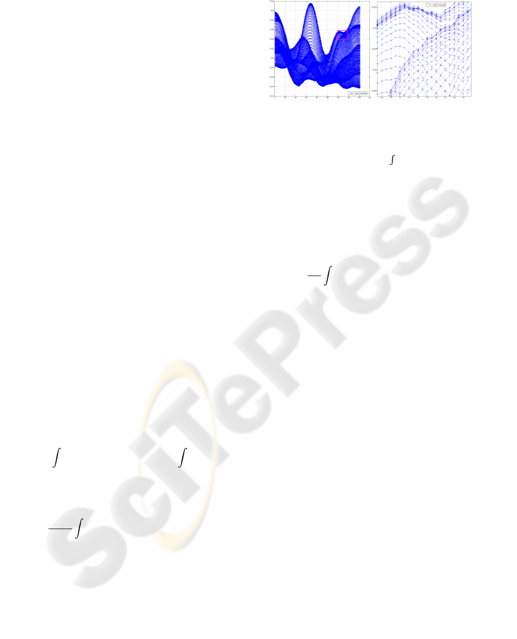
Figure 3: a|b. (a) Computed λ ∈ [0.012, 0.032] values in
sampling windows for the image with size [160, 160]. (b)
Zoom in (a) for showing the distribution of the regulariza-
tion parameters λ
w
.
noise. We note that the term
Ω
(g− hf)
2
dA is the
power of the residue. Therefore, there exists a re-
lationship among the non-oscillatory sketch “cartoon
model” (Mumford and Shah, 1989), (Blake and Zis-
serman, 1987), oscillation model (Meyer, 2001) and
the reduced power of the original image with some
proportional measure. We formulate the local vari-
ance L
w
(x,y) in a given window w based on an input
image.
L
w
(x,y) =
1
|Ω|
Ω
[ f
w
(x,y) − E( f
w
)]
2
w(x,y)dxdy (12)
where w(x, y) is a normalized and symmetric small
window, f
w
is the estimated image in a small window
w. E( f
w
) is the expected value with respect to the
window w(x, y) on the size of Ω × Ω estimated im-
age f in each iteration. The local variance in a small
window satisfies var( f
w
) = L
w
(x,y). Thereby, we can
write λ for a small window w according to Euler-
Lagrange equation for the variation with respect to f
Therefore, the regularization equation is with respect
to the window-levels. It becomes
J
ε
( f) =
∑
λ
w
L
w
(x,y) + S
p
( f) (13)
where λ
w
is a λ in a small window w, S
p
( f) is the
smoothing term. Thus, we can easily get many λ
w
for
moving windows which can be adjusted by local vari-
ances, shown in Fig. 3. These λ
w
are directly used
as regularization parameters for adjusting the balance
during the energy optimization. They also adjust the
strength of diffusion operators for keeping more fi-
delity during the diffusion process. The related regu-
larization parameters β and γ incorporate the λ, while
the parameter λ of the fidelity term needs to be de-
fined.
During image restoration, the parameter λ can be
switched among three different levels. The window-
based parameter λ
w
and the scale-based (entire im-
age) parameter can be adjusted to find the optimal
results. Simultaneously, λ thus control the image fi-
delity and diffusion strength of each selected operator
in an optimal manner.

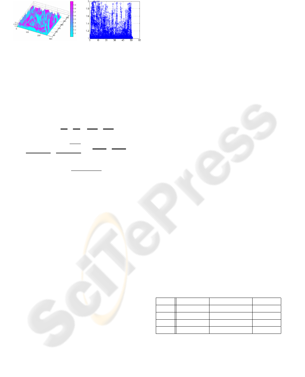
(a) (b)
Figure 4: Strength of p(x) in the Lena image. (a) Strength
of p(x) between [1,2] in the Lena image. (b) Strength of
p(x) is shown in a cropped image with size [50,50].
3.3 Data-Driven Image Diffusion
The numerical implementation is crucial for the algo-
rithm. The data-driven diffusion term div(φ(a, ∇ f))
can be numerically approximated in the following,
div(φ(x,∇ f)) = |∇f|
p(x)−2
| {z }
Coefficient
[(p(x) − 1)∆f
|
{z }
IsotropicTerm
+(2− p(x))|∇f|div(
∇f
|∇f|
)
|
{z }
CurvatureTerm
+∇p· ∇ f log|∇ f|
|
{z }
HyperbolicTerm
]
with
p(x) =

q(x) ≡ 1+
1
1+k|∇G
σ
∗I(x)|
2
, |∇f| < β
1, |∇f| ≥ β
We indicate with div the divergence operator, and
with ∇ and ∆ respectively the gradient and Laplacian
operators, with respect to the space variables. The
numerical implementation of the nonlinear diffusion
operator is based on central differences for coefficient
and the isotropic term, minmod scheme for the curva-
ture term, and upwind finite difference scheme in the
seminal work of Osher and Sethian for curve evolu-
tion (Rudin et al., 1992) of the hyperbolic term based
on the hyperbolic conservation laws. We use here the
minmod function, in order to reduce the oscillations
and to get the correct values of derivatives in the case
of local maxima and minima.
The image is restored by denoising in the pro-
cess of edge-driven image diffusion as well as deblur-
ring in the process of image deconvolution. Firstly,
the chosen variable exponent of p(x) is based on the
computation of gradient edges in the image, shown in
Fig. 4. In homogeneous flat regions, the differences
of intensity between neighboring pixels are small;
then the gradient ∇G
σ
become smaller (p(x) → 2).
The isotropic diffusion operator (Laplace) is used in
such regions. In non-homogeneous regions (near a
edge or discontinuity), the anisotropic diffusion filter
is chosen continuously based on the gradient values
(1 < p(x) < 2) of edges. The reason is that the dis-
crete chosen anisotropic operators will hamper the re-
covery of edges (Nikolova, 2004). Secondly, the non-
linear diffusion operator for piecewise image smooth-
ing is processed during image deconvolution based on
a previously estimated PSF. Finally, coupling estima-
tion of PSF (deconvolution) and estimation of image
(edge-driven piecewise smoothing) are alternately op-
timized applying a stopping criteria. Hence, over-
regularization or under-regularization is avoided by
pixels at the boundary of the restored image.
4 NUMERICAL EXPERIMENTS
Experiments on synthetic and real data are carried out
to demonstrate the effectiveness of this algorithm.
Effects of different types and strengths of noise
and blur. Firstly, we test the suggested method in dif-
ferent degraded data. Fig. 6 shows that the image de-
noising and deblurring can be successfully achieved
even on the very strong noise level SNR = 1.5dB. In
this figure, we can observe that the number of itera-
tion is dependent on the strength of noise. If the noise
is stronger, the number of iteration becomes larger.
Fig. 7 shows that the suggested approach on the BV
space is robust for different types of noise. The impul-
sive noise with different strengths can also be success-
fully eliminated, while structure and main textures are
still preserved. We have also tested this approach in
different types of noise, speckle, impulsive, Poisson,
Gaussian noise in different levels, shown in Fig. 8.
Comparison with other methods. Secondly, we
have compared the TV method with two types of con-
ditions. From visual perception and denoising view-
point, our method favorably compares to some state-
of-the-art methods: the TV method (Rudin et al.,
1992) and a wavelet method (Portilla et al., 2003).
In Fig. 5, the structure of the restored fingerprint
is largely enhanced than the original image in our
method and more recognizable in comparison with
the restored image using the GSM method (Portilla
et al., 2003).
Table 1: ISNR (dB) Results on Test Data.
SNR TV-fixed λ TV- adaptive λ Our met.
13.8 15.39 17.85 19.16
12.5 14.42 17.12 18.14
8.7 11.58 15.03 16.26
8.6 11.34 15.02 16.09
Table 1 shows the different properties of differ-
ent methods. Although our method does not have
significant improvement on the value of ISNR (dB)
in Table 1, the measure of ISNR can not fully mea-
sure human visual perception. Our method really
achieves high-fidelity and visual smoothness than the

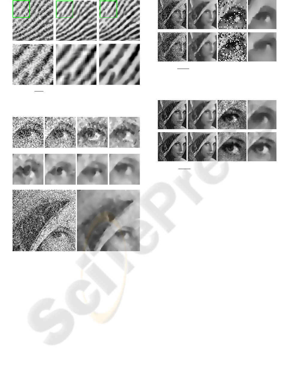
Figure 5:
a|b|c
d|e| f
. Comparison of two methods for fingerprint
denoising. (a)(d) Cropped noisy image, SNR = 8 dB. (b)(e)
GSM method (Portilla et al., 2003) PSNR=27.8. dB. (c)(f)
The suggested method PSNR= 28.6 dB.
SNR 1.5 dB 100 Iteration 200 Iteration 300 Iteration
400 Iteration 500 Iteration 550 Iteration 580 Iteration
Noise image, SNR = 1.5dB, sigma 75 Restored Image using the suggested method
Figure 6: Restored image using the suggested method.
Stronger distributed noise with SNR = 1.5dB. 100 itera-
tions need 600 seconds for the image size of [512,512].
TV methods. The TV methods with fixed λ and adap-
tive λ still have some piecewise constant effects on re-
stored images. Furthermore, our method keeps high-
fidelity for restoring stronger or impulsive noisy im-
ages, while the TV methods (fixed λ and adaptive λ)
cannot keep high-fidelity for restoring such degraded
images, e.g., SNR = 1.5dB or some impulsive noisy
images, shown in Fig. 6, Fig. 7 and Fig. 8.
More results are shown in Fig. 9 to demonstrate
that the suggested method keeps high-fidelity and vi-
sual perception image restoration. These experiments
show that the suggested method on the BV space
has some advantages on image denoising and image
Figure 7:
a|b|c|d
e| f|g|h
. Restoration of impulsive noise images.
(a) 10% salt-pepper noise image. (b) Restored image, 200
iterations. (c)(d) Zoom in images from (a)(b) respectively.
(e)25% salt-pepper noise image. (f) Restored image, 900
iterations. (g)(h) Zoom in images from (e)(f) respectively.
Figure 8:
a|b|c|d
e| f|g|h
. Image denoising using the suggested
method. (a)(b)Speckle noise image and denoising. (c)(d)
Zoom in from (a)(b) respectively, 100 iterations. (e)(f) Pois-
son noise image and denoising. (g)(h) Zoom in from (e)(f)
respectively, 100 iteration.
restoration. It can also be easily extended to other re-
lated early vision problems.
5 CONCLUSION
The main structure and skeleton of images are well
approximated on the BV space. In order to preserve
textures and detailed structures, more constraints or
generative prior information are investigated. We
have developed a self-adjusting scheme that controls
the image restoration based on the edge-driven con-
vex semi-continuous functionals. The performance
of image restoration is not only based on the com-
puted gradient but also based on local variances of
the residues. Therefore, linear and nonlinear smooth-
ing operators in the smoothing term are continuously
self-adjusting via the gradient power. The consistency
of self-adjusting local variances and the global con-
vergence can be achieved in the iterative convex op-
timization approach. We have shown that this algo-
rithm has relatively robust performance for different
types and strengths of noise. The image restoration
keeps high fidelity to the original image.

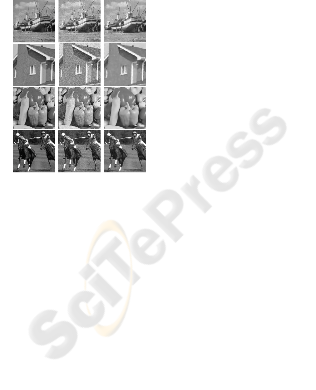
(a) (b) (c)
Figure 9: Image denoising using the suggested method. (a)
column: Original images. (b) column: Noisy images with
SNR = 10 dB . (c) column: Restored images (100 iterations)
using the suggested method.
REFERENCES
Acar, R. and Vogel, C. R. (1994). Analysis of bounded
varaition penalty methods for ill-posed problems. In-
verse problems, 10(6):1217–1229.
Alvarez, L. and Gousseau, Y. (1999). Scales in natural
images and a consequence on their bounded varia-
tion norm. In Scale-Space, volume Lectures Notes on
Computer Science, 1682.
Aubert, l. and Vese, L. (1997). A variational method
in image recovery. SIAM Journal Numer. Anal.,
34(5):1948–1979.
Blake, A. and Zisserman, A. (1987). Visual Reconstruction.
MIT Press, Cambridge.
Chambolle, A. and Lions, P. L. (1997). Image recovery
via total variation minimization and related problems.
Numer. Math., 76(2):167–188.
Chan, T. F., Kang, S. H., and Shen, J. (2002). Euler’s elas-
tica and curvature based inpaintings. SIAM J. Appli.
Math, pages 564–592.
Chan, T. F. and Shen, J. (2006). Theory and computa-
tion of variational image deblurring. Lecture Notes on
“Mathematics and Computation in Imaging Science
and Information Processing”.
Chen, Y., Levine, S., and Rao, M. (2006). Variable expo-
nent, linear growth functionals in image restoration.
SIAM Journal of Applied Mathematics, 66(4):1383–
1406.
Chen, Y. and Rao, M. (2003). Minimization problems and
associated flows related to weighted p energy and to-
tal variation. SIAM Journal of Applied Mathematics,
34:1084–1104.
Demengel, F. and Teman, R. (1984). Convex functions of a
measure and applications. Indiana University Mathe-
matics Journal, 33:673–709.
Freeman, W. and Pasztor, E. (2000). Learning low-level
vision. In Academic, K., editor, International Journal
of Computer Vision, volume 40, pages 24–57.
Geman, S. and Reynolds, G. (1992). Constrained restora-
tion and the recovery of discontinuities. IEEE Trans.
PAMI., 14:367–383.
Giusti, E. (1984). Minimal Surfaces and Functions of
Bounded Variation. Birkh
¨
auser.
Goffman, C. and Serrin, J. (1964). Sublinear functions of
measures and variational integrals. Duke Math. J.,
31:159–178.
Gousseau, Y. and Morel, J.-M. (2001). Are natural images
of bounded variation? SIAM Journal on Mathematical
Analysis, 33:634–648.
Meyer, Y. (2001). Oscillating patterns in image processing
and in some nonlinear evolution equations. The 15th
Dean Jacquelines B. Lewis Memorial Lectures, 3.
Mumford, D. and Shah, J. (1989). Optimal approximations
by piecewise smooth functions and associated varia-
tional problems. Communications on Pure and Ap-
plied Mathematics, 42:577–684.
Nikolova, M. (2004). Weakly constrained minimization:
application to the estimation of images and signals
involving constant regions. J. Math. Image Vision,
21(2):155–175.
Portilla, J., Strela, V., Wainwright, M., and Simoncelli,
E. (2003). Image denoising using scale mixtures of
Gaussians in the Wavelet domain. IEEE Trans. on
Image Processing, 12(11):1338–1351.
Rudin, L., Osher, S., and Fatemi, E. (1992). Nonlinear total
varition based noise removal algorithm. Physica D,
60:259–268.
Vese, L. A. (2001). A study in the BV space of a denoising-
deblurring variational problem. Applied Methematics
and Optimization, 44:131–161.
Weickert, J. and Schn
¨
orr, C. (2001). A theoretical frame-
work for convex regularizers in PDE-based computa-
tion of image motion. International Journal of Com-
puter Vision, 45(3):245–264.
Zheng, H. and Hellwich, O. (2006). Double regularized
Bayesian estimation for blur identification in video se-
quences. In P.J. Narayanan et al. (Eds.) ACCV, vol-
ume 3852 of LNCS, pages 943–952. Springer.