
COMPARATIVE STUDY OF CONTOUR FITTING METHODS IN
SPECKLED IMAGES
Mar´ıa E. Buemi, Juliana Gambini, Julio C. Jacobo, Marta E. Mejail
Universidad de Buenos Aires, Facultad de Ciencias Exactas y Naturales, Departamento de Computaci´on
Ciudad Universitaria, Pabell´on I, C1428EGA
Ciudad Aut´onoma de Buenos Aires – Rep´ublica Argentina
Alejandro C. Frery
Universidade Federal de Alagoas, Departamento de Tecnologia da Informac¸˜ao
BR 104 Norte km 97, 57072-970 Macei´o, AL – Brazil
Keywords:
Speckle, contour fitting, B-Spline, anisotropic diffusion, maximum likelihood.
Abstract:
Images obtained with the use of coherent illumination are affected by a noise called speckle, which is inherent
to this type of imaging systems. In this work, speckled data have been statistically treated with a multiplicative
model using the family of G distributions. One of the parameters of these distributions can be used to charac-
terize the different degrees of roughness found in speckled data. We used this information to find boundaries
between different regions within the image.
Two different region contour detection methods for speckled imagery, are presented and compared. The first
one maximizes a likelihood function over the speckled data and the second one uses anisotropic difussion over
roughness estimates. To represent detected contours, the B-Spline curve representation is used.
In order to compare the behaviour of the two methods we performed a Monte Carlo experience. It consisted
of the generation of a set of test images with a randomly shaped region, which is considered in the literature
as a difficult contour to fit. Then, the mean square error was calculated for each test image, for both methods.
1 INTRODUCTION
Several types of imaging devices employ coherent il-
lumination as, for instance, Synthetic Aperture Radar
(SAR), sonar, laser and ultrasound-B. The images
generated by these devices are affected by a noise
called speckle, a kind of degradation that does not
obey the classical hypotheses of being Gaussian and
additive. Speckle noise reduces the ability to extract
information from the data, so specialized techniques
are required to deal with such imagery.
Speckled data have been statistically modeled un-
der the multiplicative model using the family of G
distributions, since these probability laws are able to
describe the observed data better than other laws, spe-
cially in the case of rough and extremely rough areas.
As a case of interest, in SAR images such sit-
uations are common when scanning urban spots or
forests on undulated relief, and for them the more
classical Γ and K distributions do no exhibit good
performance (Frery et al., 1997; Mejail et al., 2001).
Under the G model, regions with different degrees
of roughness can be characterized by the parameters.
Therefore, this information can be used to find bound-
aries between regions with different textures.
An example is shown in Figure 1, where the
dashed lines show the ideal boundary and the solid
lines presents typical speckled data set associated to
this edge in semilogarithmic scale. As can be seen
in this figure, edge detection in speckled imagery is a
tough task due to the low signal-to-noise ratio.
0 20 40 60 80 100
0.1 0.5 1.0 5.0 10.0 50.0
Position
Boundary and Data
Figure 1: Edge (dashed lines) and speckled data (solid
lines).
309
E. Buemi M., Gambini J., C. Jacobo J., E. Mejail M. and C. Frery A. (2007).
COMPARATIVE STUDY OF CONTOUR FITTING METHODS IN SPECKLED IMAGES.
In Proceedings of the Second International Conference on Computer Vision Theory and Applications - IFP/IA, pages 309-316
Copyright
c
SciTePress

On the other hand, contours formulated by means
of B-Splines present several advantages: allow local
control, have local representation, require few para-
meters and are intrinsically smooth.
We compare two strategies for boundary detection
with B-Spline deformable contours: one that maxi-
mizes a likelihood function that directly employs the
speckled image values that obey a G
0
A
law (Gambini
et al., 2006) and another strategy that uses anisotropic
diffusion over roughness estimates based on this sta-
tistical distribution (Gambini et al., 2004).
In order to compare the behavior of both methods
we performed a Monte Carlo experience. It consists
of the generation of a set of test images with a ran-
domly shaped region. For 2D shapes of fixed perime-
ter, (Hero et al., 1999) established that disk-shaped
objects are the easiest to estimate, while flower-
shaped objects are the hardest to estimate, among the
class of objects representable by the B-Spline basis.
Then, we generate random samples obeying the G
0
A
distribution with different parameters for the points
inside and outside the flower contour. Finally, we cal-
culate the error fitting. We conclude that the maxi-
mum likelihood model assuming the G
0
A
distribution
for the speckled data is the best of these two edge de-
tection procedures with respect to both the error and
the computational cost.
The structure of this paper is as follows: section 2
describes the statistical model used for single chan-
nel speckled data, section 3 provides a brief account
of B-spline curve fitting, section 4 describes the al-
gorithms in detail, section 5 presents the error evalu-
ation methodology, section 6 presents the results and
section 7 concludes the paper.
2 THE G DISTRIBUTION FOR
SPECKLED DATA
Speckled images can be modeled as the product of
two independent random fields, one corresponding
to the backscatter X and other corresponding to the
speckle noise Y (Goodman, 1976):
Z = X ·Y. (1)
For amplitude data, the speckle noiseY is modeled
as a Γ
−1/2
(n,n) distributed random variable, where n
is the number of looks used to generate the image; this
parameter is known or estimated beforehand, and it is
valid for the whole image.
The most general model for the backscatter X here
considered is the Generalized Inverse Gaussian law
(Barndorff-Nielsen and Blaesild, 1983; Jorgensen,
1982; Seshadri, 1993), denoted as N
−1/2
(α,λ,γ).
For particular values of the parameters of the N
−1/2
distribution, the Γ
1/2
(α,λ), and the Γ
−1/2
(α,γ) distri-
butions are obtained. These, in turn, give rise to the
K
A
and the G
0
A
distributions for the return Z, respec-
tively. See(Mejail et al., 2001).
The G
0
distribution represents an attractive choice
for SAR data modeling, given its tractability, expres-
siveness and capability of retrieving detailed informa-
tion from the data (Quartulli and Datcu, 2004). Its
density function for amplitude data, is given by
f
G
0
A
(z) =
2n
n
(n− α)
γ
α
Γ(−α)Γ(n)
z
2n−1
(γ+ z
2
n)
n−α
,
−α,γ,z > 0, n ≥ 1. (2)
This situation is denoted Z ∼ G
0
A
(α,γ,n), being its
moments
E
G
0
A
(Z
r
) =
γ
2n
r/2
Γ(−α+ r/2)
Γ(−α)
Γ(n+ r/2)
Γ(n)
, (3)
if −α > r or infinite otherwise.
Speckled data is described in this paper by the G
0
A
law. Given the data, the statistical parameters are es-
timated and this information is used to extract region
boundaries present in the image.
2.1 Parameter Estimation
As presented in equation (2), the parameter α of the
G
0
A
distribution is defined for negative values. Esti-
mation is crucial in many applications and, besides
that, the value of this parameter is immediately in-
terpretable in terms of target roughness; this inter-
pretability will be treated in detail in section 2.2.
In this work sample moments parameter estima-
tion method (MO for short) is used. This technique
is based on replacing theoretical moments by sample
observations, and then calculating the unknown para-
meters.
To estimate α and γ it is necessary to estimate two
moments. In this work moments of order 1/2 and 1,
namely m
1/2
and m
1
respectively, will be used. From
equation (3), these moments are given by
m
1/2
=
γ
n
1/4
Γ(−α− 1/4)Γ(n + 1/4)
Γ(−α)Γ(n)
, (4)
m
1
=
γ
n
1/2
Γ(−α− 1/2)Γ(n + 1/2)
Γ(−α)Γ(n)
, (5)
for α < −1/4 and α < −1/2, respectively. Then, us-
ing equations (4) and (5),
b
α can be determined as the
solution of
g(
b
α) − ζ = 0, (6)
where
g(
b
α) =
Γ
2
−
b
α−
1
4
Γ(−
b
α)Γ
−
b
α−
1
2
(7)

and
ζ =
bm
2
1/2
bm
1
Γ(n)Γ(n+
1
2
)
Γ
2
(n+
1
4
)
, (8)
and then substituting the value of
b
α in equation (4)
or in equation (5) the value of
b
γ is found. It can be
noticed that g(
b
α) converges asymptotically to one as
b
α → −∞. As ζ is a random variable that can take val-
ues greater than one, there are cases for which equa-
tion (6) does not have a solution. The lower the value
of the α parameter, the higher the probability that a
solution for equation (6) does not exist. This issue
was solved by (Mejail et al., 2003) replacing unob-
served estimates by the median of surrounding values.
2.2 Parameter Interpretation
One of the most important features of the G
0
A
distrib-
ution is that the estimated values of the parameter α
have immediate interpretation in terms of roughness.
For values of α near zero, the imaged area presents
very heterogeneous gray values, as is the case of ur-
ban areas in SAR images. As we move to less hetero-
geneous areas like forests, the value of α diminishes,
reaching its lowest values for homogeneous areas like
pastures and certain types of crops. This is the reason
why this parameter is regarded to as a roughness or
texture measure.
3 B-SPLINE REPRESENTATION
We use the B-Spline curve representation for describ-
ing object contours in a scene. In the following, a
brief review of B-Spline representation of contours
is presented; for more details see (Blake and Isard,
1998) and (Rogers and Adams, 1990).
Let {Q
0
,...,Q
N
B
−1
} be a set of control points,
where Q
n
= (x
n
,y
n
)
t
∈ R
2
, 0 ≤ n ≤ N
B
− 1, and let
{s
0
< s
1
< s
2
< · · · < s
L−1
} ⊂ R be a set of L knots.
A B-Spline curve of order d is defined as a weighted
sum of N
B
polynomial basis functions B
n,d
(s) of de-
gree d − 1, within each interval [s
i
,s
i+1
] with 0 ≤
i ≤ L− 1. The spline function is r(s) = (x(s),y(s))
t
,
0 ≤ s ≤ L− 1, being
r(s) =
N
B
−1
∑
n=0
B
n,d
(s)Q
n
, (9)
and
x(s) = B
t
(s)Q
x
(10)
y(s) = B
t
(s)Q
y
(11)
where the basis functions vector B(s) of N
B
compo-
nents is given by B(s) = (B
0,d
(s),...,B
N
B
−1,d
(s))
t
.
The weight vectors Q
x
and Q
y
give the first and sec-
ond components of Q
n
, respectively.
The curves used in this work are closed, with
d = 3 or d = 4, and are specified by periodic B-Spline
basis functions.
4 BOUNDARY DETECTION
In this section we present the methods developed to
detect region boundaries in speckled imagery.
Let E be a scene made up by a background B and a
set of k distinct regions {R
1
,R
2
,...,R
k
} with bound-
aries {∂R
1
,...,∂R
k
}, respectively. Each of these re-
gions and the background are considered to be ran-
dom fields of independent, identically distributed,
random variables obeying the G
0
A
distribution and
characterized by the values of their statistical para-
meters (α
h
,γ
h
), 1 ≤ h ≤ k. The only assumption we
make is that regions and background have different
textures, i.e., if α
0
is the background roughness then
α
h
6= α
0
for every 1 ≤ h ≤ k.
For each region R
h
, we want to find the curve C
h
that fits the boundary ∂R
h
in the image. As shown
in section 2.2, there is a correspondence between the
various areas present in the image and the parameters
of roughness and scale. From this correspondence a
classification of the image can be done.
The algorithms we propose aim at separating re-
gions of a certain specified type from the rest of the
image, so we obtain a first rough approximation, or
seed: the starting regions of interest. The contour ex-
traction algorithms work over these regions instead of
analyzing the whole image reducing, thus, the com-
putational effort.
This initial region detection is computed over non-
overlapping blocks of the image using as input the
number of blocks and the type of region to be detected
(homogeneous,heterogeneous or extremely heteroge-
neous); the details are presented in (Gambini et al.,
2006). Once k regions are identified, each centroid
c
h
, 1 ≤ h ≤ k, is computed.
If a point belongs to the object boundary, then a
sample taken from its neighborhood should exhibit
a change in its properties and, therefore, could be
considered a transition point. In order to find tran-
sition points, N segments s
(i)
, 1 ≤ i ≤ N, of the form
s
(i)
=
c p
i
are considered for each region, being c the
centroid of the initial region, the extreme p
i
a point
outside of the region. It is necessary for the centroid
c to be in the interior of the object whose contour is
sought. A strip S
(i)
h
is defined over each segment s
(i)
.
This procedure is illustrated in the fluxogram of Fig-
ure 2 and in Figures 3 and 4 with a SAR image.
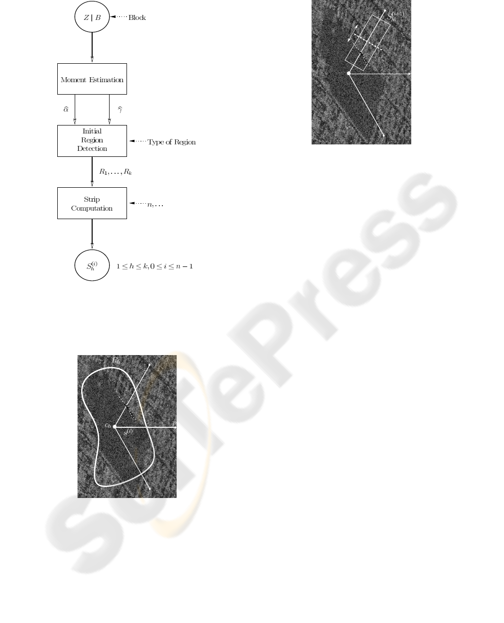
Figure 2: Sequence of operations leading from the data con-
ditioned on the blocks (Z | B) to the n strips S
(i)
h
, 0 ≤ i ≤
n−1, for each region 1 ≤ h ≤ k ≤ i ≤ n−1, for each region
1 ≤ h ≤ k.
Figure 3: Initial region R
h
with the segments s
(i)
, extreme
point p
i
and center c
h
on a SAR image.
In this work we present a comparative study of two
new methods for contour detection in speckled im-
agery using statistical properties of the data and B-
Spline curve representation. One of them uses Maxi-
mum Likelihood over speckled data and the other uses
Anisotropic Diffusion over the roughness estimates.
Figure 4: Strip S
(i+1)
h
defined over the s
(i+1)
on a SAR im-
age.
As we explain in the following section.
4.1 Maximum Likelihood (ML)
The general problem consists of finding a transition
point within each strip S
(i)
h
. These points will be
sought using the data along the discrete version of
s
(i)
, for which we will not introduce a new notation
(see Figure 2):
s
(i)
=
z
(i)
1
,...,z
(i)
m
, 1 ≤ i ≤ N. (12)
For each segment s
(i)
, 1 ≤ i ≤ N, we consider the fol-
lowing partition
Z
(i)
k
∼ G
0
A
(α
r
,γ
r
), k = 1, . .., j (13)
Z
(i)
k
∼ G
0
A
(α
b
,γ
b
), k = j + 1,...,m (14)
where for each k, with 1 ≤ k ≤ m, z
(i)
k
is the real-
ization of the random variable Z
(i)
k
. The parameters
(α
r
,γ
r
) and (α
b
,γ
b
) characterize the region and its
background, respectively.
In order to find the transition point on each seg-
ment s
(i)
, an objective functionis considered: the like-
lihood of the sample which is given by
L( j) =
j
∏
i=1
Pr(z
i
;α
r
,γ
r
) ·
m
∏
i= j+ 1
Pr(z
i
;α
b
,γ
b
). (15)
Alternatively, we can maximize
ℓ( j) = lnL( j) =
j
∑
i=1
ln( f
G
0
(z
i
;α
r
,γ
r
))
+
m
∑
i= j+ 1
ln( f
G
0
(z
i
;α
b
,γ
b
)). (16)
According to equation (2)
ℓ( j) =
∑
j
i=1
ln
2n
n
Γ(n−α
r
)z
2n−1
i
γ
α
r
r
Γ(−α
r
)Γ(n)
(
γ
r
+nz
2
i
)
n−α
r
+
+
∑
m
i= j+ 1
ln
2n
n
Γ(n−α
b
)z
2n−1
i
γ
α
b
b
Γ(−α
b
)Γ(n)
(
γ
b
+nz
2
i
)
n−α
b
. (17)
Finally, the estimated index on the segment that
corresponds to the transition point
b
j is given by
b
j = argmax
j
ℓ( j). (18)
The scheme of this procedure is shown in Algo-
rithm 1.
Algorithm 1 Edge detection by maximum likelihood
using raw data.
1: for each segment s
(i)
, i = 1,... , N do
2: Estimate the parameters (α
r
,γ
r
) and (α
b
,γ
b
).
3: Find the index
b
j on the segment s
(i)
that maxi-
mizes equation (18); it corresponds to the bor-
der point b
i
in the image.
4: end for
5: Build the B-Spline curve that interpolates the
boundary points {b
1
,...,b
N
}.
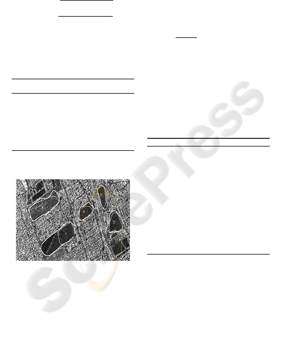
In Figure 5 the result of applying algorithm 1 to a
real SAR image, is shown.
Figure 5: Maximum likelihood edge detection in a SAR
image of Munich.
4.2 Anisotropic Diffusion (AD)
Another way of finding the transition point on a line
s
(i)
is to estimate the α parameter in a window cen-
tered on each pixel on the line using the data on the
strip S
(i)
. Then an array
b
Λ
(i)
= [
b
α
(i)
1
,...,
b
α
(i)
m
] of esti-
mates of the α parameter is obtained. If a point lies
on the boundary between two regions, then it exhibits
an abrupt change in the values of the α estimates.
(Perona and Malik, 1990) proposed an algorithm
that combats noise preserving boundary features. In
its continuous version, it consists of producing a se-
quence of images I(·,·,t), t ≥ 0, according to the fol-
lowing equation:
∂I(x,y,t)
∂t
= ∇· [g(k∇Ik)∇I], (19)
where I(·,·,0): R
2
→ R
+
is the original image, t is
an artificial time parameter, ∇I is the image gradient,
k∇Ik is the image gradient magnitude, ‘∇ · ’ denotes
the divergence, g: R → [0, 1] is an edge detection
function with the only constraints that (i) g(x) → 0
monotonically when x → ∞, and (ii) g(x) → 1 when
x → 0. More details can be found in, among others,
(Weickert, 1998).
The position of the discontinuity on s
(i)
is found
by convolving the smoothed roughness estimates with
a cyclic border detection operator, followed by a con-
venient thresholding. The scheme of this procedure is
shown in Algorithm 2.
Algorithm 2 Edge detection by anisotropic diffusion.
1: for each segment s
(i)
, i = 1,... , N do
2: Estimate the parameter α for each pixel on s
(i)
using a sliding window. This generates an ar-
ray
b
Λ
(i)
= [
b
α
(i)
1
,...,
b
α
(i)
m
] of estimated values of
α.
3: Smooth the array
b
Λ
(i)
using anisotropic diffu-
sion. This generates the smoothed estimates
array
b
Λ
(i)
S
.
4: Find b
i
, the position on line s
(i)
that corre-
sponds to the maximum discontinuity among
the values in the smoothed array
b
Λ
(i)
S
convolv-
ing with the mask [−2,−1, 0,1,2].
5: end for
6: Build the B-Spline curve that interpolates the
boundary points {b
1
,...,b
N
}.
In Figure 6, the results of applying Algorithm 2,
are shown. Having proposed two edge detection tech-
niques, we now proceed to their comparative assess-
ment.
5 CONTOUR FITTING ERROR
This section is devoted to the study of the error com-
mitted in the determination of contours by applying
the segmentation methods described above to a series
of randomly generated images.
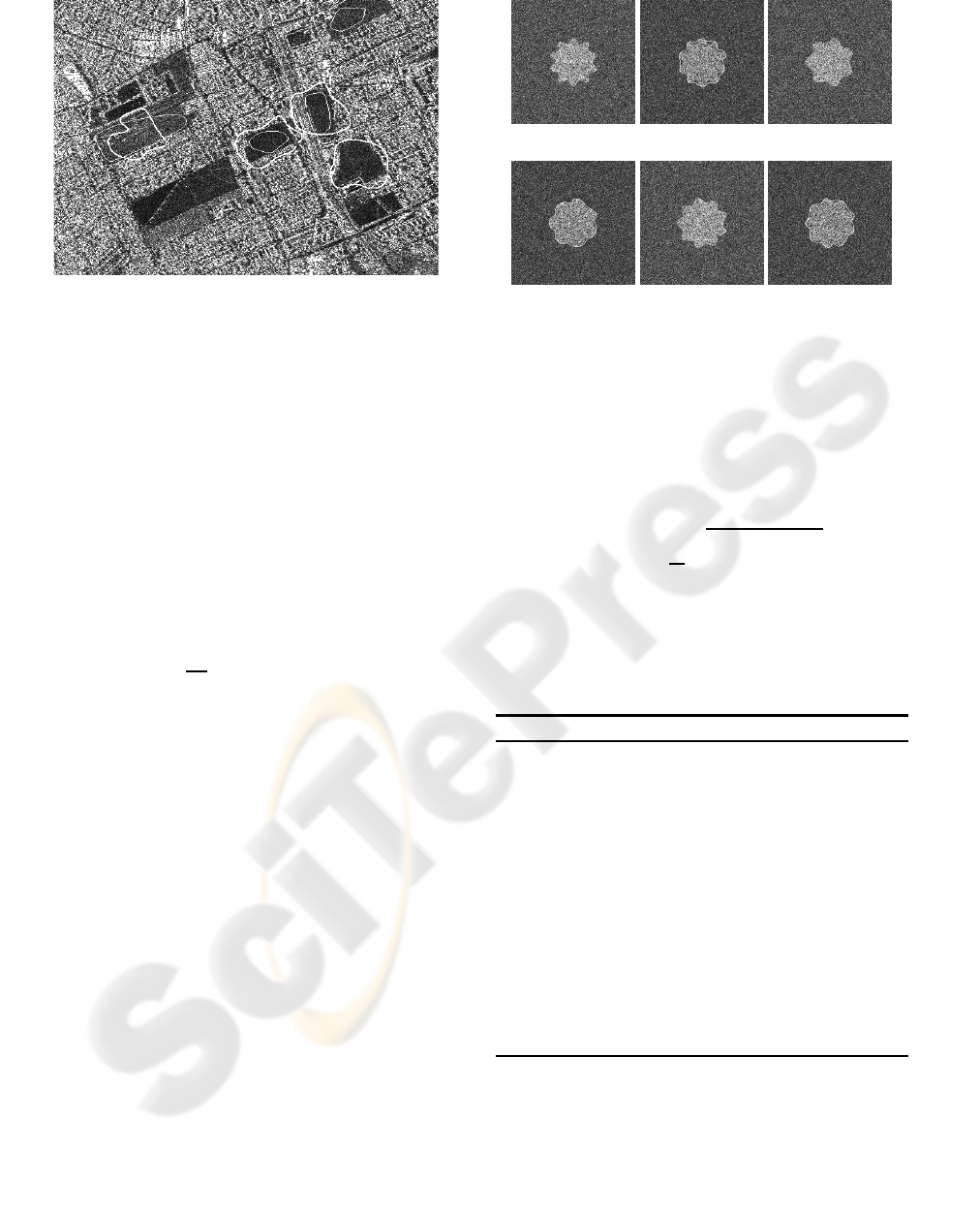
Figure 6: Edge detection by anisotropic detection in a SAR
image of Munich.
The error evaluation algorithm is applied to a fam-
ily of synthetic random images of flower shaped re-
gions {F
k
}
k=1,...,n
. Then, the error of approximating
these regions by the obtained B-Spline curves is es-
timated. The {F
k
}
k=1,...,n
are formed in two stages:
first a random region is generated, and then the back-
ground and foreground are simulated.
The random region boundary is generated accord-
ing to a parametric curve in polar coordinates given
by
f(s;η,β,δ) = (θ(s),ρ(s;η,β,δ)), s ∈ [0,S]
θ(s) = s
2π
S
ρ(s;η,β,δ) = η− δcos(βθ(s)),
(20)
where η is the flower radius, β is the number of petals
and 2δ is the petal depth.
In this work the parameters η, β and δ are considered
to be independent random variables uniformly distrib-
uted the sets [5,20], {15,...,50} and [2, 10], respec-
tively.
After a region boundary is generated, G
0
A
dis-
tributed speckle noise is added to the image. Fig-
ure 7shows some of these simulated images, along
with the estimated boundaries.
In order to calculate the error in boundary fitting
we consider ∂R to be the boundary of the region to be
segmented and C the resulting curve. Let s
1
,...,s
m
be
a set of radial lines given by s
j
= λ~u
j
+ c j = 1...m,
where ~u
j
is a unitary vector that determines the line
direction, and c is the centroid of region R. The point
c and the vectors ~u
j
j = 1,...,m are the same for all
of the test images. Let
~
V
j
be the intersection points
between curve C and line s
j
, and let
~
W
j
be the inter-
section points between curve ∂R and the line s
j
:
s
j
∩ C =
~
V
j
, s
j
∩ ∂R =
~
W
j
. (21)
(a) (b) (c)
(d) (e) (f)
Figure 7: Synthetic images and detected boundaries with
maximum likelihood method: (a) Image F
1
with η = 10,
β = 45, δ = 6, (b) Boundary curve F
1
, (c) Image F
2
with
η = 7, β = 46, δ = 5, (d) Boundary curve F
2
, (e) Image F
3
with η = 9, β = 48, δ = 5 and (f) Boundary curve F
3
.
The distance between C and ∂R can be then defined
as
d(∂R,C) =
1
N
v
u
u
t
N
∑
j= 1
~
V
j
−
~
W
j
2
, (22)
where N is the number of segments. This is a measure
of the error committed when estimating ∂R by C .
Algorithm 3 shows the procedure for calculating
the error.
Algorithm 3 Contour Fitting Error.
1: Generate a set of test images using equation (20)
and the G
0
A
distribution.
2: for each method do
3: for each image do
4: Find the fitting curve for the flower contour
through the method in evaluation.
5: for j = 0,...,N do
6: Find the points
~
V
j
and
~
W
j
, using equa-
tion (21).
7: Find the distance as in equation (22).
8: end for
9: Return d(∂R,C).
10: end for
11: end for
With the error values calculated in Algorithm 3 for
each of the test images, a graphic that serves as an aid
for the comprehension of each method and that allows
for comparisons between the two methods, is done.
Let e
max
be the maximum error incured when ap-
plying this method. Let us consider the error interval
[0,e
max
] and let partition it as {e
0
,...,e
m
}, so
e
i
= e
0
+ ∆ ∗ i, i = 0,...,m (23)
where m is such that e
max
= e
0
+ ∆ ∗ m and ∆ is the
partition length. We define the histogram function h :
[0,e
max
] → N such that
h(e
i
) = #{F
k
:e
i
≤ d(∂R
k
,C
k
) < e
i+1
}, i = 0,...,m−1.
(24)
We call h
M
the function h calculated after applying
the method M. We say that a method is efficient if the
valuesof h are high for values close to zero. We define
function h
A
: [0,e
max
] → N, by
h(e
i
) = #{F
k
: d(∂R,C) ≤ e
i
}, i = 0,...,m− 1, (25)
We call h
M
A
the accumulated histogram function
calculated for method M. A method M is more effi-
cient than another method K if, for a given error value
e
i
, the condition
h
M
A
(e
i
) > h
K
A
(e
i
) (26)
holds.
A Monte Carlo experience was conducted in or-
der to assess the error committed by our proposal, us-
ing 108 simulated images according to the aforemen-
tioned model.
6 RESULTS
In this section, the error committed in the Maximum
Likelihood and Anisotropic Diffusion methods, is es-
timated. A Monte Carlo experience was conducted
in order to assess the error committed by our pro-
posal. We generated 108 simulated images with data
obeying the G
0
A
(α,1,1) distribution, with parameters
α = −3 for the flower and α = −10 for the back-
ground. Then, the contour fitting error is calculated
using Algorithm 3, as explained in section 5.
The result for each method is an array of values
corresponding to the error committed in each test im-
age. Then, functions h
M
(e
i
) and h
M
A
(e
i
), i = 0, ... , m
using equations (24) and (25), respectively, are calcu-
lated.
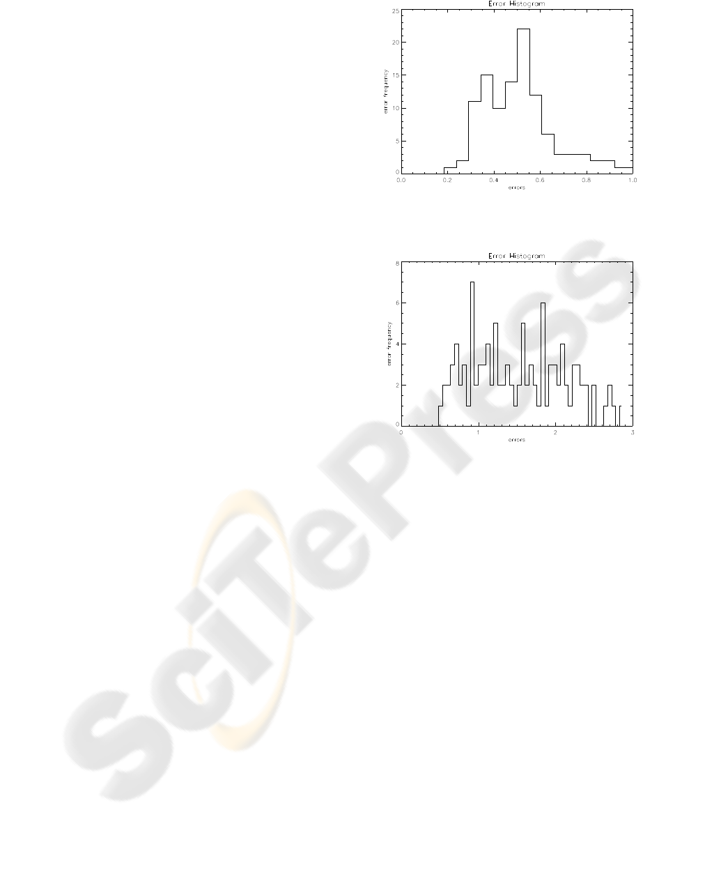
Figures 8 and 9 show the error histograms h
M
(e
i
)
for the methods ML and AD, respectively. In both
graphics, the horizontal axis corresponds to the error
intervals, and the vertical axis indicates the number of
images with error within each interval.
In order to visualize the comparison between the
errors for both methods, Figure 10 depicting their er-
ror histograms, is shown.
The error values shown here are between 0.0 and
1.0 because the values near zero are of more inter-
est. It is observed that, for the ML method, most of
Figure 8: Error histogram for the ML method.
Figure 9: Error histogram for the AD method.
the images have error values less than 0.6, while for
the AD method, most of the images have error values
greater than 1.0. In section 7, conclusions based on
these graphics are derived about the behavior of both
methods.
In Figure 11 the accumulated error h
M
A
(e
i
) , given
by equation 25, is shown for both methods. In this
graphic it can be seen that there are 81 images with
error below 1.0 for the ML method, while for the AD
method there are only 26 images in that condition. It
can also be seen that
h
ML
A
(e) > h
AD
A
(e) (27)
for e < 1.7.
7 CONCLUSIONS
The goal of this paper was to compare two contour
detection methods for speckled data: Maximum Like-
lihood, performed over the raw data, and Anistropic
Diffusion, over estimates of the α parameter of the
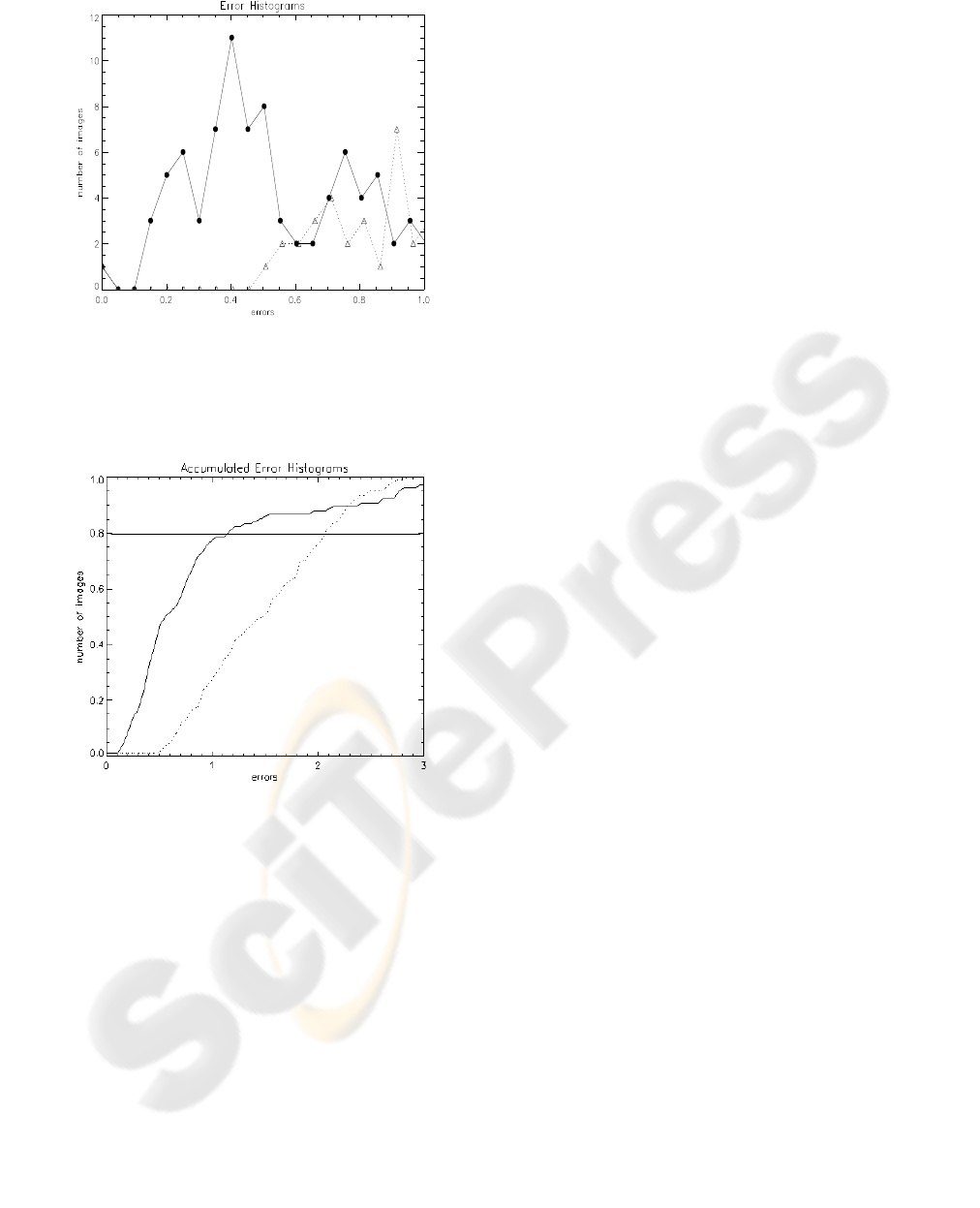
Figure 10: Error histograms for each method: the contin-
uous line with bullets ’•’ corresponds to the ML method,
and the dashed line with the triangles ’△’ corresponds to
the AD method.
Figure 11: Accumulated errors for both methods: continu-
ous line ML method, dashed line AD method. The horizon-
tal line indicates 80% level.
G
0
A
distribution. To this end, a Monte Carlo expe-
rience was conducted in which a region pattern was
randomly generated and then it was submitted to both
boundary fitting algorithms. The error values for the
methods under study was then calculated.
In Figure 11 we observe that in the case of
the Maximum Likelihood method, 80% of the seg-
mented images have errors below 1.1, and that for the
Anisotropic Diffusion method, 80% of the segmented
images have errors below 1.8. This indicates that the
first boundary fitting method is better than the second.
Regarding the computational cost, it was also ob-
served that Maximum Likelihood was significantly
faster than Anisotropic Diffusion.
REFERENCES
Barndorff-Nielsen, O. E. and Blaesild, P. (1983). Hiperbolic
Distributions. Kotz and Johnson eds., Encyclopedia of
Statistical Science, Wiley, 3:700–707.
Blake, A. and Isard, M. (1998). Active Contours. Springer
Verlag.
Frery, A. C., M¨uller, H.-J., Yanasse, C. C. F., and
Sant’Anna, S. J. S. (1997). A model for extremely het-
erogeneous clutter. IEEE Transactions on Geoscience
and Remote Sensing, 35(3):648–659.
Gambini, J., Mejail, M., Berlls, J. J., and Frery, A. (2006).
Feature extraction in speckled imagery using dynamic
b-spline deformable contours under the G
0
models.
IJRS International Journal of Remote Sensing. to ap-
pear.
Gambini, M. J., Mejail, M., Jacobo-Berlles, J. C., Muller,
H., and Frery, A. C. (2004). Automatic contour detec-
tion in SAR images. In Proceedings EUSAR04.
Goodman, J. W. (1976). Some Fundamental Properties of
Speckle. Journal of the Optical Society of America,
66:1145–1150.
Hero, A. O., Piramuthu, R., Fessler, J. A., and Titus, S. R.
(1999). Minimax emission computed tomography us-
ing high-resolution anatomical side information and
b-spline models. IEEE Transactions on Information
Theory, 45(3):920–938.
Jorgensen, B. (1982). Statistical Properties of the General-
ized Inverse Gaussian Distribution. Lecture Notes in
Statistic, Springer-Verlag, 9.
Mejail, M., Jacobo-Berlles, J. C., Frery, A. C., and Bustos,
O. H. (2003). Classification of SAR images using a
general and tractable multiplicative model. Interna-
tional Journal of Remote Sensing, 24(18):3565–3582.
Mejail, M. E., Frery, A. C., Jacobo-Berlles, J., and Bus-
tos, O. H. (2001). Approximation of distributions for
SAR images: Proposal, evaluation and practical con-
sequences. Latin American Applied Research, 31:83–
92.
Perona, P. and Malik, J. (1990). Scale-space and edge detec-
tion using anisotropic diffusion. IEEE Trans. Pattern
Anal. Machine Intell., 12(7):629–639.
Quartulli, M. and Datcu, M. (2004). Stochastic geomet-
rical modelling for built-up area understanding from
a single SAR intensity image with meter resolution.
IEEE Transactions on Geoscience and Remote Sens-
ing, 42(9):1996–2003.
Rogers, D. F. and Adams, J. A. (1990). Mathematical El-
ements for Computer Graphics. McGraw-Hill, New
York, USA, 2 edition.
Seshadri, V. (1993). The Inverse Gaussian Distribution:
A Case of Study in Exponential Families. Claredon
Press, Oxford, first edition.
Weickert, J. (1998). Anisotropic Diffusion in Image
Processing. Teubner-Verlag, first edition.
