
AN UNSUPERVISED SONAR IMAGES SEGMENTATION
APPR
OACH
Abdel-Ouahab Boudraa
IRENav, Ecole Navale & E
3
I
2
, (EA 3876) ENSIETA
Lanv
´
eoc Poulmic, BP600, 29200 Brest−Arm
´
ees, France
Jean-Christophe Cexus
IUT de Lannion
BP 30219, Rue Edouard Branly 22302 Lannion Cedex, France
Keywords:
Image segmentation, Gabor filtering, Clustering, Feature selection, Texture, Sonar image.
Abstract:
In this work an unsupervised Sonar (Sound navigation and ranging) images segmentation is proposed. Due to
the textural nature of the Sonar images, a band-pass filtering that takes into account the local spatial frequency
of these images is proposed. Sonar image is passed through a bank of Gabor filters and the filtered images
that possess a significant component of the original image are selected. To calculate the radial frequencies, a
new approach is proposed. The selected filtered images are then subjected to a non-linear transformation. An
energy measure is defined on the transformed images in order to compute texture features. The texture energy
features are used as input to a clustering algorithm. The segmentation scheme has been successfully tested on
real high-resolution Sonar images, yielding very promising results.
1 INTRODUCTION
Synthetic aperture side scan Sonar imagery has long
been a field of intense research interest for both mili-
tary and civilian applications. An example of applica-
tion is the sea mine detection and classification where
traditionally a human operator would be required to
carry out the analysis based on its expert knowledge.
In high resolution Sonar imagery, three kinds of re-
gion can be visualized: echo, shadow, and sea-bottom
reverberation. On images supplied by Sonar system,
the echo features are generally less discriminant than
the shadow shapes for the classification of objects ly-
ing on the sea-bed. For this reason, the detection of
each object located on the sea bottom and its classi-
fication (as a wreck, a rock, a man-made object, etc.)
is generally based on the extraction and the identifi-
cation of its cast shadow (Collet et al., 1996). A num-
ber of unsupervised techniques have been proposed to
segment Sonar images, including use of Markov Ran-
dom Fields (MRF) to approximate the differing gray
level regions and pixel correlations within the regions
(Murino, 2001)-(Mignotte et al., 1999). The later
technique provides an accurate segmentation, but is
computationally intense. A fuzzy clustering method
has recently been proposed to the segmentation prob-
lem using gray level information (Stitt et al., 2001).
However, fuzzy clustering is very sensitive to speckle
noise. Due the textural nature of the Sonar images and
to the fact that they are strongly corrupted by speckle
noise, a multi-channel filtering approach is suitable to
take into account the local spatial frequency content
of these images and to reduce the noisy components.
In this work Gabor filters (Gabor, 1946) are used as
band-pass filters (Daugman, 1985). Gabor kernels are
commonly used for texture feature extraction. Their
popularity is motivated by the mathematical and the
biological properties of Gabor functions.
2 FILTER BANK DESIGN
Gabor filters provide simultaneous optimal resolution
in both space and spatial-frequency domains (Daug-
man, 1985). In spatial domain, the complex impulse
response of Gabor filters is given by
h(x,y) = exp
−
1
2
(x−x
0
)
2
r
σ
2
x
+
(y−y
0
)
2
r
σ
2
y
×
exp
2πj(µ
0
x+ ν
0
y)
(1)
165
Boudraa A. and Cexus J. (2007).
AN UNSUPERVISED SONAR IMAGES SEGMENTATION APPROACH.
In Proceedings of the Second International Conference on Computer Vision Theory and Applications - IFP/IA, pages 165-170
Copyright
c
SciTePress

h(x,y) is a complex sinusoid, known as the carrier,
centered at the spatial frequency (µ
0
,ν
0
) in Cartesian
coordinates and modulated by a 2D Gaussian-shaped
function, known as the envelope. σ
x
and σ
y
are the
space constants of the Gaussian envelope along the
x and y axes, respectively. µ
0
and ν
0
are the central
radial frequencies along the x and y directions respec-
tively. These spatial frequencies can also be expressed
in polar coordinates as (F
0
,θ):
µ
0
= F
0
cosθ and ν
0
= F
0
sinθ (2)
F
0
is the radial center frequency measured in cycles
per pixel. The point (x
0
,y
0
) is he peak of the function
h(x,y), and r subscript sands for a rotation operation
such that
(x−x
0
)
r
(y−y
0
)
r
=
cosθ sinθ
−sinθ cosθ
.
x−x
0
y−y
0
(3)
Filter with an arbitrary orientation, θ, can be obtained
via the rigid rotation of the x −y coordinates system
using relation (3). The angle θ is also the angle of
rotation of the envelope. The 2-D Fourier transform,
or spectral transfer function, of the real part of the
Gabor function is given by (even-symmetric filters):
H(u,v) = A
exp
−
1
2
(u−u
0
)
2
r
σ
2
u
+
v
2
r
σ
2
v
+exp
−
1
2
(u+u
0
)
2
r
σ
2
u
+
v
2
r
σ
2
v
!
(4)
where A = 2πσ
x
σ
y
, and (u, v) are the components of
the frequency in the x and y directions respectively.
σ
u
= 1/2πσ
x
, σ
v
= 1/2πσ
y
are the extents of the
Gaussian envelope in the spectral domain in the x and
y directions respectively.
3 SELECTION OF PARAMETERS
By passing the original image through a Gabor filter,
we obtain all those components in the image that have
their energies concentrated near the spatial frequency
point (±u
0
) within a frequency bandwidth of B
r
oc-
taves and orientation bandwidth of B
θ
degrees. A Ga-
bor filter bank is usually designed to cover all avail-
able the frequency spectrum (Jain and Farrokhnia,
1991),(Manjunath and Ma, 1996),(Guo et al., 2000).
In general the Gabor filter set is constructed such that
the half-peak magnitude (η = 0.5) of the filter in the
frequency spectrum touch each other. In this work, we
define the η-peak magnitude of the filter to compute
B
r
as follows:
B
r
= 2log
2
µ
0
+
p
(−2lnη)σ
u
µ
0
−
p
(−2lnη)σ
u
(5)
where η ∈ [0,1] is the filter magnitude where neigh-
boring filters along the µ axis intersect. To calcu-
late radial frequencies, a new approach, different than
that proposed by (Jain and Farrokhnia, 1991), is pre-
sented. Let f
l
and f
h
be the lower and the higher fre-
quency respectively (u
0
(0) = u
0
∈ [ f
l
, f
u
]). We sup-
pose that the radial frequencies follows a logarithmic
scale and the frequencies of the i
th
and (i-1)
th
filters
are such that:
u
0
(i)
u
0
(i−1)
= 2
B
r
andB
r
=
ln(
f
l
f
u
)
nln2
(6)
In the frequency domain the spread σ
u
(i) and σ
v
(i) of
the i
th
filter are given by:
σ
u
(i) = 2
i×B
r
andσ
v
(i) =
K
b
K
a
.σ
u
(i)
K
b
= tan
π
2K
θ
andK
a
=
2
B
r
−1
2
B
r
+1
(7)
where σ
v
(0) = σ
0
and K
θ
is the number of orienta-
tions.
4 MULTI-CHANNEL FILTERING
For an original image I(x,y), the output of the Gabor
filter, I
h
(x,y) is given by
I
h
(x,y) = I(x, y) ∗h(x,y) (8)
where ∗ denotes the convolution product. The image
I(x,y) is filtered using a bank of L = n ×K
θ
filters
where n is the number of scales used. The n value
can be given by the number of radial frequencies
µ
0
used or the width of the image, N. Thus, if
N is a power of 2, the frequencies selected are:
1
√
2,2
√
2,4
√
2,8
√
2,...,(N/4)
√
2 cycles per width.
The filters orientation (θ ∈ [0,π]) is given by
θ
m
= m
π
K
θ
with m ∈ {0,1,...,K
θ
−1} (9)
The angular bandwidth, B
θ
, is given by
B
θ
=
π
K
θ
(10)
Before generating the feature images, each filtered
image is transformed in a new image, I
NL
(x,y), using
a non-linear function:
I
NL
(x,y) = ψ(α | I
h
(x,y) |) (11)
where
ψ(t) = tanh(αt) =
1−exp(−2αt)
1+ exp(−2αt)
(12)

where α is a constant (Jain and Farrokhnia, 1991)
(α = 0.25 is this study). A texture measure is de-
fined over a small Gaussian window, with a standard
deviation σ =
N
2F
0
and of size M ×M, around each
transformed pixel in the selected filtered images. M
is inversely related to u
0
, and is the smallest odd in-
teger larger than or equal to 5σ, where σ = 0.25N/u
0
(Jain and Farrokhnia, 1991). More formally, the fea-
ture image e
k
(x,y), corresponding to the k
th
filtered
image r
k
(x,y), is given by
e
k
(x,y) =
1
M
2
∑
(a,b)∈W
xy
| ψ((r
k
(a,b)) | (13)
where W
xy
is a window of size M
2
centered at pixel
(x,y).
5 SPACE REDUCTION
The values in the L feature images corresponding to a
given pixel form an L-dimensional feature vector rep-
resenting the pixel. Features are normalized to zero
mean and unit standard deviation. Some filtered im-
ages may show similar response to different textures
because the textures may share the same spatial fre-
quency properties. Hence, the L filtered images are
not all of practical interest and thus space reduction is
necessary to discard irrelevant image features. Prin-
cipal Components Analysis (PCA) is commonly used
reduction technique (Jolliffe, 1986). Given a set of
data, PCA finds the linear lower-dimensional repre-
sentation of the data such that the variance of the re-
constructed data is preserved. Intuitively, PCA finds
a low-dimensional hyperplane such that, when we
project the data onto the hyperplane, the variance of
the data is changed as little as possible (maximum of
data variance). In general there is no standard rule
for deciding how many principal components should
be used to represent the data adequately, but a useful
heuristic is to choose a fraction (0.8 in this study) of
the inertia I
q
to be retained by computing:
I
q
=
q≤p
∑
j=1
λ
j
p
∑
i=1
λ
i
(14)
λ
j
denotes eigenvalues and p denotes the number of
eigenvalues.
6 CLUSTERING
K-means is well known method for clustering data
(Jain and Dubes, 1988). However, like all partitional
algorithms, the k-means requires the number of clus-
ters before starting the clustering process. Due to
the low contrast and the speckle of Sonar images,
the estimation of the number of clusters is very dif-
ficult (Figs. 2(a),9(a),10(a)). To avoid this problem
the k-means is started with an overestimated number
of clusters, KC, and combined with the dendrogram
(Jain and Dubes, 1988).
7 RESULTS
Experiments have been conducted on real Sonar im-
ages (Figs. 2(a),9(a),10(a)). Sonar images are pro-
vided by a side-scan Sonar with frequency around 500
kHz. The size of these images is 256×256 pixels cor-
responding to a sea floor surface of 25 by 25 m. Thus,
for N = 256 a filter bank can be created with a to-
tal of n = 7 central frequencies or scales associated
to a given orientation. The number of orientations K
θ
is set to 5. Finally, we start with L = 35 Gabor fil-
ters. For each pixel (x, y) is associated a feature vec-
tor of 35 features. Using the dendrogram the num-
ber of clusters is reduced to 2. Figure 2(a) displays
a man made object (Trolley) lying on the sea bed.
Gaobr filter with tuned radial frequency and orienta-
tions is applied to ”Trolley” image (Fig. 2(a)). Figure
3 shows 20 filtered images (among 35) correspond-
ing to five orientations: 0
◦
, 36
◦
, 72
◦
, 108
◦
, 144
◦
. The
filtered images clearly show that filter responses in
object-echo regions are different from those in the non
object-echo regions. Feature images are obtained by
transforming the filtered images using a non-linearly
relation (Eq. 11) followed by a Gaussian filtering (Eq.
13). Result of 15 feature images is shown in figure
4. Not that the feature values corresponding to ob-
ject (Trolley) are consistently high. A PCA analysis
performed for space reduction is shown in figure 5.
This figure shows that many feature images are irrel-
evant and this is confirmed by the calculated eigen-
values 7. Indeed, the plot of figure 7 shows that most
the information of the original image (”Trolley”) is
concentrated on few eigenvalues and thus only a re-
duced number of feature images is of practical in-
terest. From the reduced number of feature images,
feature vectors are formed and clustered using the
k-means with KC set to 10. Result of clustering is
shown in figure 6. Figure 8 shows the dendrogram
obtained using the KC cluster centers generated by
the k-means. The extracted shadow of the trolley ex-

hibits, as expect, a regular shape (Fig. 2(b)). Figure
9(a) displays a real Sonar image of sandy floor with
the cast shadow of a manufactured object (cylinder).
As in Figure 2, the shadow region est well segmented
(Fig. 9(b)). Figure 10(a) displays a real Sonar image
involving an object and rock shadows. The segmen-
tation result is shown in figure 10(b). The shadows
of the rock and the manufactured object are well de-
tected. However, a post processing such as connected
components analysis is necessary to the two shad-
ows. The obtained results (Figs. 2(b),9(b),10(b)) are
in good agreement with the ground truth provided by
an expert. Note that figures 2(c), 9(c) and 10(c) dis-
play the class or cluster corresponding to set formed
by echo and sea-bottom reverberation. The accuracy
in extracting and preserving the borders of the cast
shadows is very appealing in the prospect of as further
classification step. Furthermore the proposed scheme
exhibits good robustness against speckle noise.
8 CONCLUSIONS
In this paper an unsupervised segmentation method to
distinguish, from Sonar images, man-made and natu-
ral objects lying on the sea-bed is presented. The ob-
tained results show the interest of multi-channel fil-
tering, based on the Gabor filters, to segment Sonar
images. To calculate the radial frequencies of the Ga-
bor filters a new approach is proposed. To confirm the
obtained results a large of Sonar images to segment is
necessary. Furthermore, we plan to study the influ-
ence of the number of Gabor filters on detection ob-
jects on sea floor followed with a ROC analysis (False
alarm,....). Finally, comparison of the obtained results
to those of existing methods and particularly those
based one the Markovian model (Mignotte et al.,
1999) in terms of time complexity and False alarm
is necessary.
ACKNOWLEDGMENTS
The authors would like to thank GESMA (Groupe
d’
´
Etude Sous Marine de l’Atlantique), Brest, France
for providing real Sonar images.
REFERENCES
Collet, C., Thourel, P., Perez, P., and Bouthemy, P. (1996).
Hierarchical mrf modeling for sonar picture segmen-
tation. In Proc. IEEE ICIP, pages 979–982.
Daugman, J. (1985). Uncertainty relation for resolution in
space, spatial frequency, and orientation optimized by
two-dimensional visual cortical filters. J. Opt. Soc.
Amer., 2:1160–1169.
Gabor, D. (1946). Theory of communication. J. Inst. Elect.
Eng., 93:429–457.
Guo, G., Li, S., Chan, K., and Pan, H. (2000). Texture
image segmentation using reduced gabor filter set and
mean shift clustering. In Proc. of the Fouth Asian Con-
ference on Computer Vision.
Jain, A. and Dubes, R. (1988). Algorithms for clustering
data. Prentice Hall, New Jersey.
Jain, A. and Farrokhnia, F. (1991). Unsupervised texture
segmentation using gabor filters. Pattern Recognition,
24(12):1167–1186.
Jolliffe, I. (1986). Principal Component Analysis. Springer-
Verlag, New York.
Manjunath, B. and Ma, W. (1996). Texture features for
browsing and retrieval of image data. IEEE Trans-
actions on Pattern Analysis and Machine Intelligence,
18:937–842.
Mignotte, M., Collet, C., Perez, P., and Bouthemy, P.
(1999). Three class markovian segmentation of high
resolution sonar images. Computer Vision Image Un-
derstanding, 76(3):191–204.
Murino, V. (2001). Reconstruction and segmentation of
underwater acoustic images combining confidence
information in mrf models. Pattern Recognition,
34(5):981–997.
Stitt, J., Tutwiler, R., and Lewis, A. (2001). Fuzzy c-means
image segmentation of side scan sonar images. In
Proc. IASTED.
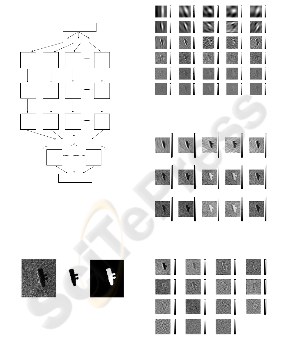
Space Reduction
Energy
Computation
Bank of Gabor Filters
Input Image
Feature
Images
Nonlinearity
Filtered
Images
Response
Images
Segmented Image
Clustering
Figure 1: Overview of the segmentation process.
Figure 2: A real Sonar image involving sea floor and a
man-made object (trolley) (a:left image). Extracted cluster
”Shadow” (b: middle image). Complement of the cluster
”Shadow” (c: right image).
0
0.5
1
1: 0°,Fo: 1.6105
0
0.5
1
2: 36°,Fo: 1.6105
0
0.5
1
3: 72°,Fo: 1.6105
0
0.5
1
4: 108°,Fo: 1.6105
0
0.5
1
5: 144°,Fo: 1.6105
0
0.5
1
6: 0°,Fo: 3.5767
0
0.5
1
7: 36°,Fo: 3.5767
0
0.5
1
8: 72°,Fo: 3.5767
0
0.5
1
9: 108°,Fo: 3.5767
0
0.5
1
10: 144°,Fo: 3.5767
0
0.5
1
11: 0°,Fo: 7.9434
0
0.5
1
12: 36°,Fo: 7.9434
0
0.5
1
13: 72°,Fo: 7.9434
0
0.5
1
14: 108°,Fo: 7.9434
0
0.5
1
15: 144°,Fo: 7.9434
0
0.5
1
16: 0°,Fo: 17.6416
0
0.5
1
17: 36°,Fo: 17.6416
0
0.5
1
18: 72°,Fo: 17.6416
0
0.5
1
19: 108°,Fo: 17.6416
0
0.5
1
20: 144°,Fo: 17.6416
0
0.5
1
21: 0°,Fo: 39.1804
0
0.5
1
22: 36°,Fo: 39.1804
0
0.5
1
23: 72°,Fo: 39.1804
0
0.5
1
24: 108°,Fo: 39.1804
0
0.5
1
25: 144°,Fo: 39.1804
0
0.5
1
26: 0°,Fo: 87.016
0
0.5
1
27: 36°,Fo: 87.016
0
0.5
1
28: 72°,Fo: 87.016
0
0.5
1
29: 108°,Fo: 87.016
0
0.5
1
30: 144°,Fo: 87.016
Figure 3: Example of 20 filtered images for Trolley image.
0
0.5
1
16: 0°,Fo: 17.6416
0
0.5
1
17: 36°,Fo: 17.6416
0
0.5
1
18: 72°,Fo: 17.6416
0
0.5
1
19: 108°,Fo: 17.6416
0
0.5
1
20: 144°,Fo: 17.6416
0
0.5
1
21: 0°,Fo: 39.1804
0
0.5
1
22: 36°,Fo: 39.1804
0
0.5
1
23: 72°,Fo: 39.1804
0
0.5
1
24: 108°,Fo: 39.1804
0
0.5
1
25: 144°,Fo: 39.1804
0
0.5
1
26: 0°,Fo: 87.016
0
0.5
1
27: 36°,Fo: 87.016
0
0.5
1
28: 72°,Fo: 87.016
0
0.5
1
29: 108°,Fo: 87.016
0
0.5
1
30: 144°,Fo: 87.016
Figure 4: Example of 15 Feature images.
0
0.5
1
direction: 1
0
0.5
1
direction: 2
0
0.5
1
direction: 3
0
0.5
1
direction: 4
0
0.5
1
direction: 5
0
0.5
1
direction: 6
0
0.5
1
direction: 7
0
0.5
1
direction: 8
0
0.5
1
direction: 9
0
0.5
1
direction: 10
0
0.5
1
direction: 11
0
0.5
1
direction: 12
0
0.5
1
direction: 13
0
0.5
1
direction: 14
0
0.5
1
direction: 15
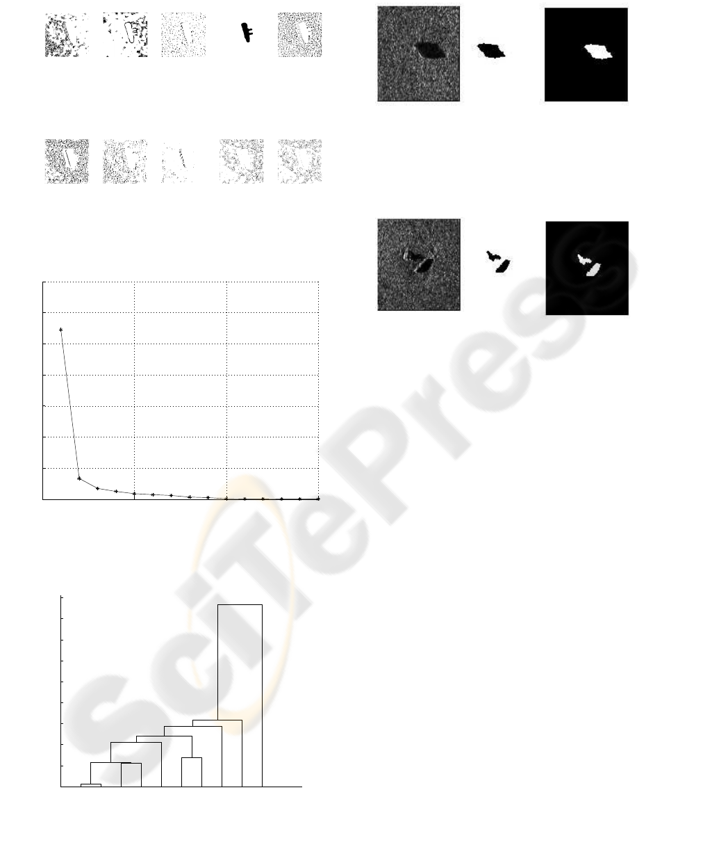
Figure 5: ACP analysis.
classe: 1 classe: 2 classe: 3 classe: 4 classe: 5
classe: 6 classe: 7 classe: 8 classe: 9 classe: 10
Figure 6: Clustering using 10 classes of Trolley image.
0 5 10 15
0
0.1
0.2
0.3
0.4
0.5
0.6
0.7
valeurs propres
Figure 7: Eigenvalues.
0
0.2
0.4
0.6
0.8
1
1.2
1.4
1.6
1.8
9 10 6 7 2 1 5 3 8 4
Dendrogram
Figure 8: An example of dendrogram obtained using the
cluster centers generated by the k-means.
Figure 9: A real Sonar image of a sandy sea floor with the
shadow of a man-made object (cylinder) (a:left image). Ex-
tracted cluster ”Shadow” (b: middle image). Complement
of the cluster ”Shadow” (c: right image).
Figure 10: A real Sonar image involving an object and a
rock shadows (a:left image). Extracted cluster ”Shadow”
(b: middle image). Complement of the cluster ”Shadow”
(c: right image).
