
AUTOMATED STAR/GALAXY DISCRIMINATION IN
MULTISPECTRAL WIDE-FIELD IMAGES
Jorge de la Calleja
Instituto Nacional de Astrof
´
ısica,
´
Optica y Electr
´
onica, Santa Mar
´
ıa Tonantzintla, Puebla, M
´
exico
Olac Fuentes
Computer Science Department, University of Texas at El Paso, El Paso, Texas, U.S.A.
Keywords:
Image Analysis, Machine Learning, Imbalanced Datasets.
Abstract:
In this paper we present an automated method for classifying astronomical objects in multi-spectral wide-
field images. The classification method is divided into three main stages. The first one consists of locating
and matching the astronomical objects in the multi-spectral images. In the second stage we create a compact
representation of each object applying principal component analysis to the images. In the last stage we classify
the astronomical objects using locally weighted linear regression and a novel oversampling algorithm to deal
with the unbalance that is inherent to this class of problems. Our experimental results show that our method
performs accurate classification using small training sets and in the presence of significant class unbalance.
1 INTRODUCTION
Currently, several multi-band astronomical surveys,
such as the Sloan Digital Sky Survey
1
, the Two Mi-
cron All Sky Survey
2
, and the Digitized Palomar Ob-
servatory Sky Survey
3
, are producing enormous im-
age databases that require automated tools for any
kind of analysis. Analyzing wide-field images has
been and still is of great importance in astrophysics:
from studies of the structure and dynamics of our
Galaxy, to galaxy formation and evolution, to the
large scale structure of the Universe (Andreon et al.,
2000).
Recently, there has been a great deal of inter-
est from astronomers in applying computer vision
and pattern recognition techniques to solve astronom-
ical image analysis problems. Examples of these
works include classification of galaxies (Bazell and
Aha, 2001; DelaCalleja and Fuentes, 2004; Lahav,
1996; Naim et al., 1995; Owens et al., 1996; Storrie-
Lombardi et al., 1992), stars (Bailer-Jones et al.,
1998), binary stars (Weaver, 2000), star/galaxy dis-
crimination (Andreon, 1999; M ¨ahonen and Hakala,
1
http://www.sdss.org
2
http://www.ipac.caltech.edu/2mass
3
http://dposs.ncsa.uiuc.edu
1995; Philip et al., 2002) and many others. Some
works have started using multi-spectral images, for
example, Zhang and Zhao used data from the optical,
X-ray, and infrared bands to classify active galactic
nuclei (AGN), stars, and galaxies, using learning vec-
tor quantization, support vector machines and single-
layer perceptrons (Zhang and Zhao, 2004).
In general, the first steps in analyzing astronom-
ical images are the detection and classification of
the objects in them. This presents significant chal-
lenges in the case of multi-spectral images, as as-
tronomical objects have widely varying appearances
at different wavelengths. In this work we propose
a method to classify astronomical objects in multi-
spectral wide-field images in a fully automated man-
ner. This method first locates and matches the ob-
jects in the different multi-spectral images. Then, it
creates a new representation for each object using its
multi-spectral images. After that, it employs princi-
pal component analysis to reduce the dimensionality
of the data and to find relevant information. Finally,
it uses locally weighted linear regression to classify
the objects. Since most astronomical problems in-
volve large degrees of class unbalance (for example in
our galaxy/star discrimination problem, galaxies out-
number stars by a factor of 10), we also introduce a
method to deal the problem of imbalanced data sets.
155
de la Calleja J. and Fuentes O. (2007).
AUTOMATED STAR/GALAXY DISCRIMINATION IN MULTISPECTRAL WIDE-FIELD IMAGES.
In Proceedings of the Second International Conference on Computer Vision Theory and Applications - IU/MTSV, pages 155-160
Copyright
c
SciTePress
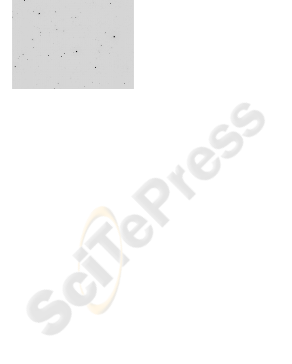
Figure 1: An astronomical wide-field image taken in the
infrared band.
The paper is organized as follows: in Section 2 we
give a brief introduction about multi-spectral wide-
field images in Astronomy. In Section 3 we describe
the method for classifying the astronomical objects,
including its main three components. Next, in Sec-
tion 4, we introduce our proposed method for dealing
with imbalanced data sets. Section 5 presents exper-
imental results. Some conclusions and directions of
future research are presented in Section 6.
2 MULTI-SPECTRAL
WIDE-FIELD IMAGES
An astronomical wide-field image (see Figure 1) nor-
mally contains from tens to thousands of objects.
These objects may be stars, galaxies, nebulas, or
quasars, among others. Multi-spectral imaging refers
to acquiring several images of the same scene using
different spectral bands. The spectral distribution of
celestial sources carries essential information about
the physical processes that take place in these ob-
jects (Nuzillard and Bijaoui, 2000). Generally, multi-
spectral images provide more information than a sin-
gle wavelength one.
The final goal in processing multi-spectral wide-
field images is usually to construct catalogues that
contain astrometric, geometric, morphological and
photometric parameters for each object in the image
(Andreon, 1999).
3 THE CLASSIFICATION
METHOD
The method we present to classify the astronomical
objects is divided into three main stages. The first
one consists of locating and matching the astronom-
ical objects among the multi-spectral images. In the
second stage we create a new representation for each
object using its multi-spectral images, and also we
find a set of features using principal component analy-
sis. Finally, in the last task we classify the astronomi-
cal objects using locally weighted linear regression in
combination with an oversampling algorithm to deal
with the class unbalance inherent to this problem. The
following subsections describe in detail these tasks.
3.1 Location and Matching of the
Astronomical Objects
First, for each multi-spectral image I we separate the
objects from background applying a threshold as fol-
lows
S(i, j) =
I(i, j), if I(i, j) ≥ threshold;
0, otherwise.
(1)
where S is the segmented image, and (i, j) repre-
sent a position in the image.
Then, we locate the astronomical objects in the
segmented images. We can locate an object by the
coordinates (x
1
,y
1
,x
2
,y
2
) of the bounding rectangle
that encloses it. Our algorithm for locating objects
is based on the flood-fill algorithm (Hearn and Baker,
1997). The purpose of flood fill is to color an entire
area of connected pixels with the same color.
We assume that all the pixels that appear different
from the background correspond to astronomical ob-
jects. Thus, our algorithm proceeds as follows: We
examine every location in the image, then when we
find a pixel different from the background, we search
its neighbors, i.e. we search its neighbors in the right,
left, up and down directions, and mark these pixels.
We store the positions of these neighbors to examine
again their neighbors. When we find a left neighbor
and its position x
1
is smaller than the previous one,
we will change it. We do the same for y
1
, x
2
and
y
2
, but considering up, right and down, respectively.
This process is repeated until the image is fully ex-
amined. In the end we will have located each object
in each of the multi-spectral images by its coordinates
(x
1
,y
1
,x
2
,y
2
). In Table 1 we outline the algorithm to
locate objects, and in Figure 2 we show an example
of location of objects.
We select some of the located objects according to
their size, i.e. if the objects are larger than a threshold
we will select them. We do this selection process be-
cause many objects are very small, two or three pixels
of size.
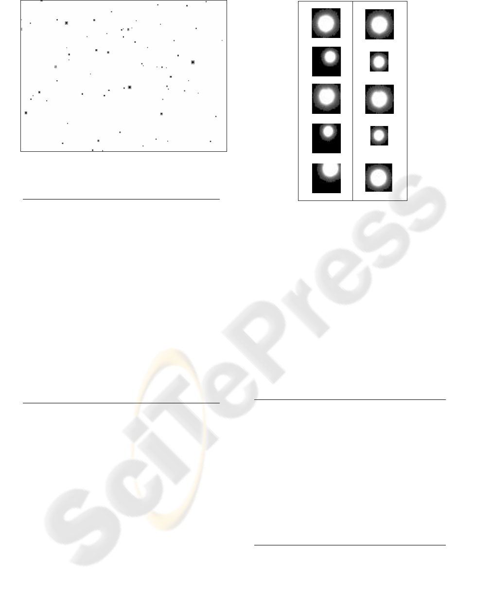
Figure 2: The located objects are marked by a rectangle.
Table 1: The algorithm to locate the astronomical objects.
S is the segmented image, with r rows and c columns
N is the set of neighbors, initially empty
For i = 1 to r
For j = 1 to c
If S(i, j) 6= background and is not marked
- x
1
= j
- y
1
= i
- x
2
= j
- y
2
= i
- N = (i, j)
while N 6= ⊘ do:
- Find the right, left, up
and down neighbors of (i, j)
- Add to N the neighbors of (i, j)
- if it is necessary
Modify (x
1
,y
1
,x
2
,y
2
)
- Mark S(i, j) and its neighbors
- Erase marked neighbors in N
endwhile
endfor
endfor
Most of the time a single object does not appear
in exactly the same location in the different multi-
spectral images. This can be due to slight misalign-
ments in the imaging system, tracking errors in the
telescope, or actual differences in appearance of the
object at different wavelengths. Also, these objects
may appear in different sizes or they may not even ap-
pear at all at some wavelengths. Therefore, we have
to devise an algorithm to robustly identify the same
object in the different multi-spectral images.
The idea of our algorithm to match objects is the
following: We search the largest object among the
multi-spectral images. Then, we use its coordinates
(x
1
,y
1
,x
2
,y
2
) to find the same object, but in the other
images. Almost always the object may not appear ex-
actly in the same position, then we use the Euclidean
distance to match the closest object to our interest
point. Sometimes we may not match any object be-
(a)(b)
Figure 3: Column (a) shows an object in the different multi-
spectral images. We can see that this one is not located in
the same position. Column (b) shows the same object after
matching.
cause in the images may appear only black pixels; in
these cases we assign as match point the location of
the largest object. This process is repeated until all
the objects have been matched. Because we match
an object in five multi-spectral images, we will have
five representations of the same object. Table 2 sum-
marizes our algorithm to match objects and Figure 3
shows an example of matching.
Table 2: The algorithm to match the astronomical objects.
Γ is the set of multi-spectral images
while Γ contains objects to match do:
- Find G, the largest object in Γ
- Obtain p
g
, the coordinate where G was found
- Obtain r
g
, the region that encloses G
- Obtain Γ
g
, the image where G was found
- Q = Γ − Γ
g
- Search G in Q
- Let q = (x
c
,y
r
) be the coordinates
of the objects in Q
- Find the closest objects to p
g
with q using the Euclidean distance
- ∆ = the matched objects
- Erase the matched objects in Γ
endwhile
3.2 Extracting Features
Once we have located and matched the astronomical
objects in the multi-spectral images, we crop each ob-
ject in the original image set to create our data set.
g u i z r
m
n
Vectors
ofsize m nx
mxn
5
Objectinthefivebands
Newrepresentationofanobject
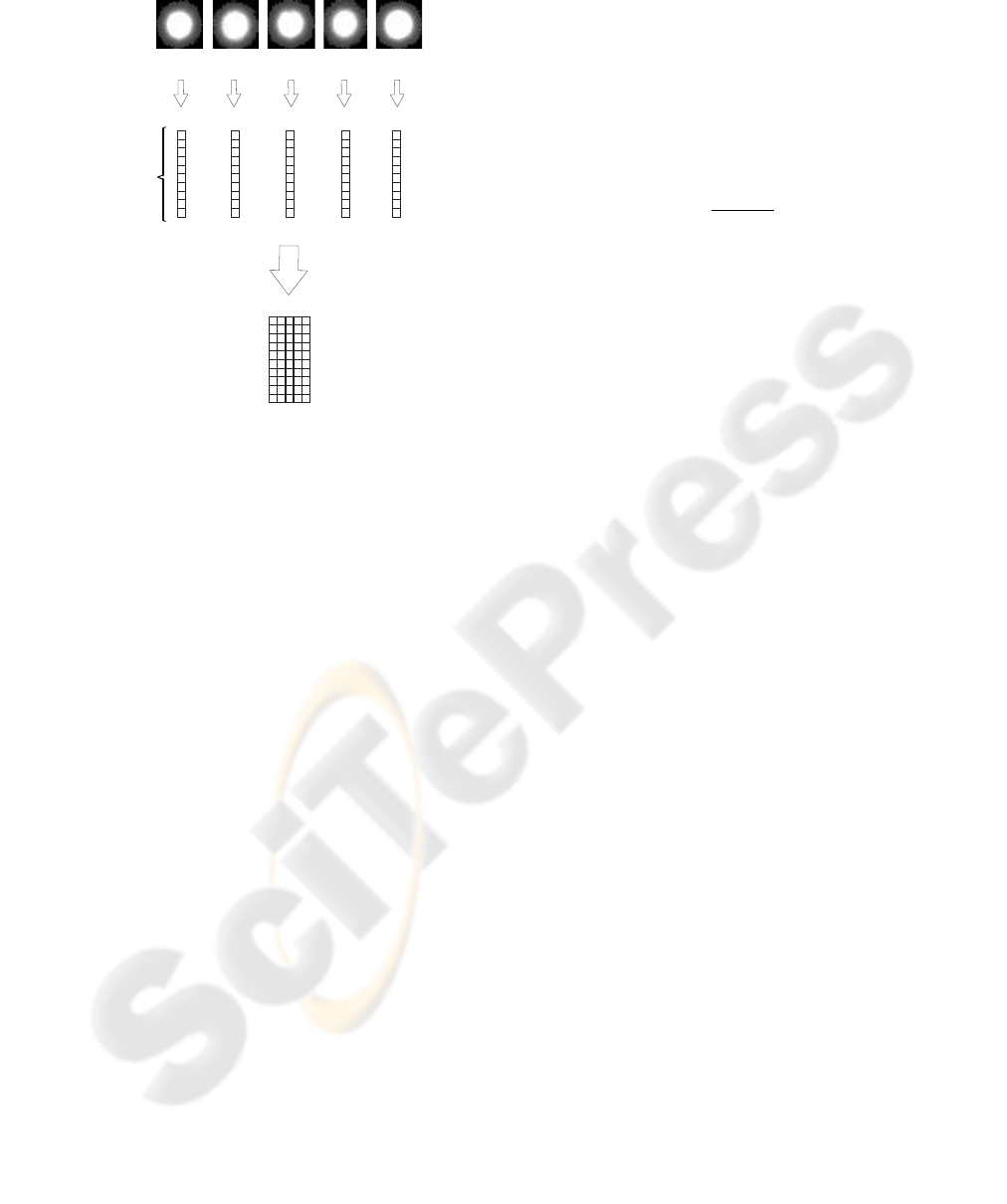
Figure 4: Process to create a new object representation.
Again, we use the coordinates (x
1
,y
1
,x
2
,y
2
) of each
object to crop it.
Each object has five representations, according to
the different bands u, g, r, i and z. Each m× n image at
each wavelength is converted into a vector of length
mn, then, these vectors are concatenated to create a
matrix of size of m × n × 5, i.e. the size of the vec-
tor by the number of multi-spectral representations.
In figure 4 we show the process of creating this new
representation.
Because we have a large data set, we use princi-
pal component analysis (PCA) to reduce its dimen-
sionality and also to find features (principal compo-
nents) that permit us to classify the astronomical ob-
jects. Details about PCA can be found in (Turk and
Pentland, 1991).
3.3 Classifying Objects
Finally, we use locally weighted linear regression
(LWLR) to classify the astronomical objects. This
machine learning algorithm takes as input parameters
the projection of the new representation of the ob-
jects onto a few set of principal components. Next,
we briefly describe this method.
3.3.1 Locally Weighted Linear Regression
Locally-weighted regression belongs to the family of
instance-based learning methods. These kinds of al-
gorithms simply store all training examples, and when
they have to classify new instances, they find similar
examples to them. In this work we use a linear model
around the query point to approximate the target func-
tion.
Given a query point x
q
, to predict its output pa-
rameters y
q
, we assign to each example in the training
set a weight given by the inverse of the distance from
the training point to the query point:
w
i
=
1
|x
q
− x
i
|
(2)
Let W, the weight matrix, be a diagonal matrix
with entries w
1
,. ..,w
n
. Let X be a matrix whose rows
are the vectors x
1
,. ..,x
n
, the input parameters of the
examples in the training set, with the addition of a ”1”
in the last column. Let Y be a matrix whose rows are
the vectors y
1
,. ..,y
n
, the output parameters of the ex-
amples in the training set. Then the weighted training
data are given by Z = WX and the weighted target
function is V = WY. Then we use the estimator for
the target function defined as:
y
q
= x
T
q
Z
∗
V (3)
where Z
∗
is the pseudoinverse of Z.
4 THE METHOD TO DEAL
IMBALANCED DATA SETS
The class imbalance problem occurs when there are
many more examples of some classes than others,
such as in our case, where we have more examples
of stars than galaxies. Two main approaches have
been used in machine learning to deal with class im-
balance. The first consists of assigning distinct costs
to training examples, weighting more heavily those in
the minority class (Pazzani et al., 1994; Domingos,
1999). The second approach is to re-sample the origi-
nal dataset, either by over-sampling the minority class
and/or under-sampling the majority class (Japkowicz,
2000; Kubat and Matwin, 1997; Chawla et al., 2002).
Our method follows the second approach, and is
similar to the SMOTE (Chawla et al., 2002) algo-
rithm, i.e. the minority class is over-sampled by tak-
ing each minority class sample and adding synthetic
examples in the original data. The purpose of aug-
manting the minority class is to create a balanced data
set, which helps to improve results in the classifica-
tion task.
Our method generates the synthetic examples as
follows: First we separate positive and negative ex-
amples from the original data set, then we find the n

Table 3: The algorithm to create new examples.
D is the original data set
N is the set of negative examples
P = D− N
for each example E in P
- Find the n closest examples to E
using the weighted distance
- Obtain A, the average of n
- δ = E - A
- η = E + δ ∗ σ(0,1)
Add η to D
endfor
closest examples to each positive (minority) example
using the weighted distance and taking into account
only the positive data set. Then we average these n
closest instances, take the difference between each
minority example (under consideration) and the av-
erage instance, multiply this difference by a random
number between 0 and 1, and add it to the original
data set. Table 4 outlines our oversampling algorithm.
5 EXPERIMENTAL RESULTS
We tested our method using images taken in five
wavelengths: u, g, r, i and z, i.e. one in ultraviolet,
one using the green filter, one using the red filter, and
two infrared, respectively. These images are of size of
1489×2048 pixels and were obtained from the Sloan
Digital Sky Survey. We used two data sets, the first
one (DB1) contained 62 stars and 7 galaxies, and the
the second one (DB2) had 141 stars and 28 galaxies.
These objects were labeled by hand, i.e. we examine
each image and assign a label to each object.
We used 3 principal components that represent
about 90% of the original information in the data sets.
We implemented locally weighted linear regression
and the over-sampling method in Matlab
TM
.
In all the experiments reported here we used 10-
fold cross-validation. Also, we vary the amount for
over-sampling from 0% to 1000%. The results we
show later correspond to the average of five runs.
We evaluated our method using two metrics: pre-
cision and recall. This metrics can be defined as fol-
lows:
Recall = TP/(TP+ FN) (4)
Precision = TP/(TP+FP) (5)
Where TP denotes the number of positive exam-
ples that are classified correctly, while FN and FP
Table 4: The table below show the results for the first data
set (DB1) using different amount for over-sampling.
0% 100% 200% 400% 1000%
Recall .343 .400 .343 .485 .542
Precision .486 .530 .500 .474 .607
Table 5: The table below show the results for the second
data set (DB2) using different amount for over-sampling.
0% 100% 200% 400% 1000%
Recall .692 .757 .750 .742 .742
Precision .740 .789 .774 .771 .667
denote the number of misclassified positive and nega-
tive examples, respectively.
In Table 4 we show the results for the first data
set (DB1). We can observe that the best results are
obtained when we use 1000% for over-sampling, i.e.
.542 and .607 for recall and precision, respectively.
In Table 5 we show the results for the second data set
(DB2). Here we can see that better results are ob-
tained than using DB1. This may be due to the fact
that we have more examples to train our classifier.
Also, the best results were obtained using only 100%
for over-sampling, with .757 for recall and .789 for
precision.
6 CONCLUSION
We have presented a method for classifying astro-
nomical objects in multi-spectral wide-field images
in a fully automated manner. Also, we introduced a
method to deal with imbalanced data sets that permits
to improve classification results. Our results are com-
parable with the best reported in the literature, but we
are using significantly smaller training sets, thus bet-
ter results should be expected when we experiment
with larger data sets. Current and future work in-
cludes: testing the method for classifying more types
of astronomical objects, using larger data sets, and
testing the oversampling method on standardized data
sets.
ACKNOWLEDGEMENTS
The first author wants to thank CONACyT for sup-
porting this research under grant 166596.

REFERENCES
Andreon, S. (1999). Neural nets and star/galaxy separation
in wide field astronomical images. In Proceedings of
International Joint Conference on Neural Networks.
Andreon, S., Gargiulo, G., Longo, G., Tagliaferri, R., and
Campuano, N. (2000). Wide field imaging - i. ap-
plications of neural networks to object detection and
star/galaxy classification. Monthly Notices of the
Royal Astronomical Society, 319:700–716.
Bailer-Jones, C., C.A.L., Irwin, M., and von Hippel, T.
(1998). Automated classification of stellar spectra. ii:
Two-dimensional classification with neural networks
and principal components analysis. Monthly Notices
of the Royal Astronomical Society, 298:361.
Bazell, D. and Aha, D. (2001). Ensembles of classifiers for
morphological galaxy classification. The Astrophysi-
cal Journal, 548:219–233.
Chawla, N., Bowyer, K., Hall, L., and Kegelmeyer, P.
(2002). Smote: Synthetic minority over-sampling
technique. Journal of Artificial Intelligence Research,
16:321–357.
DelaCalleja, J. and Fuentes, O. (2004). Machine learning
and image analysis for morphological galaxy classi-
fication. Monthly Notices of the Royal Astronomical
Society, 349:87–93.
Domingos, P. (1999). Metacost: A general method for mak-
ing classifiers cost-sensitive. In Proceedings of the
5th International Conference on Knowledge Discov-
ery and Data Mining, pages 155–164.
Hearn and Baker (1997). Computer Graphics. Prentice
Hall, 2nd. edition.
Japkowicz, N. (2000). The class imbalance problem: Sig-
nificance and strategies. In Proceedings of the 2000
International Conference on Artificial Intelligence
(IC-AI’2000): Special Track on Inductive Learning,
pages 111–117.
Kubat, M. and Matwin, S. (1997). Addressing the curse of
imbalanced training sets: One sided selection. In Pro-
ceedings of the Fourteenth International Conference
on Machine Learning, pages 179–186.
Lahav, O. (1996). Artificial neural networks as a tool for
galaxy classification. In Proceedings in Data Analysis
in Astronomy.
M¨ahonen, P. and Hakala, P. (1995). Automated source clas-
sification using a kohonen network. The Astrophysical
Journal, 452:L77–L80.
Naim, A., Lahav, O., Sodr
´
e, L., Jr, and Storrie-Lombardi,
M. (1995). Automated morphological classification of
apm galaxies by supervised artificial neural networks.
Monthly Notices of the Royal Astronomical Society,
275:567.
Nuzillard, D. and Bijaoui, A. (2000). Blind source sepa-
ration and analysis of multispectral astronomical im-
ages. Astronomy and Astrophysics, 147:129.
Owens, E., Griffiths, R., and Ratnatunga, K. (1996). Us-
ing oblique decision trees for the morphological clas-
sification of galaxies. Monthly Notices of the Royal
Astronomical Society, 281:153.
Pazzani, M., Merz, C., Murphy, P., Ali, K., Hume, T., and
Brunk, C. (1994). Reducing misclassification costs. In
Proceedings of the Eleventh International Conference
on Machine Learning, pages 217–225.
Philip, N., Wadadekar, Y., Kembhavi, A., and Joseph, K.
(2002). A difference boosting neural network for au-
tomated star-galaxy classification. Astronomy and As-
trophysics, 385:1119–1126.
Storrie-Lombardi, M., Lahav, O., Sodr
´
e, L., Jr, and Storrie-
Lombardie, L. (1992). Morphological classification
of galaxies by artificial neural networks. Monthly No-
tices of the Royal Astronomical Society, 259:8.
Turk, M. and Pentland, A. (1991). Eigenfaces for recogni-
tion. Journal of Cognitive Neuroscience, 3(1):71–86.
Weaver, B. (2000). Spectral classification of unresolved bi-
nary stars with artificial neural networks. The Astro-
physical Journal, 541:298–305.
Zhang, Y. and Zhao, Y. (2004). Automated clustering algo-
rithms for classification of astronomical objects. The
Astrophysical Journal, 422:1113–1121.
