A SPATIAL SAMPLING MECHANISM FOR EFFECTIVE
BACKGROUND SUBTRACTION
Marco Cristani and Vittorio Murino
Computer Science Dep., Universit
`
a degli Studi of Verona, Strada Le Grazie 15, Verona, Italy
Keywords:
Background subtraction, mixture of Gaussian, video surveillance.
Abstract:
In the video surveillance literature, background (BG) subtraction is an important and fundamental issue. In
this context, a consistent group of methods operates at region level, evaluating in fixed zones of interest pixel
values’ statistics, so that a per-pixel foreground (FG) labeling can be performed. In this paper, we propose a
novel hybrid, pixel/region, approach for background subtraction. The method, named Spatial-Time Adaptive
Per Pixel Mixture Of Gaussian (S-TAPPMOG), evaluates pixel statistics considering zones of interest that
change continuously over time, adopting a sampling mechanism. In this way, numerous classical BG issues
can be efficiently faced: actually, it is possible to model the background information more accurately in the
chromatic uniform regions exhibiting stable behavior, thus minimizing foreground camouflages. At the same
time, it is possible to model successfully regions of similar color but corrupted by heavy noise, in order to
minimize false FG detections. Such approach, outperforming state of the art methods, is able to run in quasi-
real time and it can be used at a basis for more structured background subtraction algorithms.
1 INTRODUCTION
Background subtraction is a fundamental step in auto-
mated surveillance. It represents a pixel classification
task, where the classes are the background (BG), i.e.,
the expected part of the monitored scene, and the fore-
ground (FG), i.e., the interesting visual information
(e.g., moving objects). As witnessed by the related
literature (see Sect.2), choosing the right class can-
not be adequately performed by per pixel methods,
i.e., considering every temporal pixel evolution as an
independent process. Instead, region based methods
better behave, deciding the class of a pixel value by
inspecting the related neighborhood.
In this paper, we propose a novel approach for
background subtraction which constitutes a per region
extension of a widely used and effective per pixel BG
model, namely the Time Adaptive Per Pixel Mixture
Of Gaussian (TAPPMOG) model. The proposed ap-
proach, called Spatial-TAPPMOG (S-TAPPMOG), is
based on a sampling mechanism, inspired by the par-
ticle filtering paradigm. The goal of the approach is to
provide a per pixel characterization of the BG which
takes into account selectively for contributions com-
ing from the neighboring pixel locations. The result
is constituted by a set of per pixel models which are
built per region: this characterization turns out to be
very robust to false FG alarms, especially when the
scene is heavily cluttered, and in general highly robust
to the FG misses (i.e., not detected FG pixel values).
In particular, several problems that classically affect
BG subtraction schemes are successfully faced by the
proposed method. Theoretical considerations and ex-
tensive comparative experimental tests prove the ef-
fectiveness of the proposed approach.
The rest of the paper is organized as follows. Section
2 reviews briefly the huge BG subtraction literature.
In Section 3, the needed mathematical fundamentals,
i.e., the TAPPMOG model and the particle filtering
paradigm, are reported. The whole strategy is detailed
in Section 4, and, finally, in Section 5, experiments on
real data validate our method and conclude the paper.
403
Cristani M. and Murino V. (2007).
A SPATIAL SAMPLING MECHANISM FOR EFFECTIVE BACKGROUND SUBTRACTION.
In Proceedings of the Second International Conference on Computer Vision Theory and Applications - IU/MTSV, pages 403-410
Copyright
c
 SciTePress

2 STATE OF THE ART
The actual BG subtraction literature is large and mul-
tifaceted; here we propose a taxonomy in which the
BG methods are organized in i) per pixel, ii) per re-
gion, iii) per frame and iv) hybrid methods. Note that
our approach is located in the hybrid method class.
The class of per pixel approaches is formed by meth-
ods that perform BG/FG discrimination by consider-
ing each pixel signal as an independent process. One
of the first BG modeling was proposed in the surveil-
lance system Pfinder ((Wren et al., 1997)), where
each pixel signal was modeled as a uni-modal Gaus-
sian distribution. In ((Stauffer and Grimson, 1999)),
the pixel evolution is modeled as a multimodal sig-
nal, described with a time-adaptive mixture of Gaus-
sian components (TAPPMOG). Another per-pixel ap-
proach is proposed in ((Mittal and Paragios, 2004)):
this model uses a non-parametric prediction algorithm
to estimate the probability density function of each
pixel, which is continuously updated to capture fast
gray level variations. In ((Nakai, 1995)), pixel value
probability densities, represented as normalized his-
tograms, are accumulated over time, and BG label are
assigned by MAP criterion.
Region based algorithms usually divide the frames
into blocks and calculate block-specific features;
change detection is then achieved via block match-
ing, considering for example fusion of edge and in-
tensity information ((Noriega and Bernier, 2006)). In
((Heikkila and M.Pietikainen, 2006)) a region model
describing local texture characteristic is presented;
the method is prone to errors when shadows and sud-
den global changes of illumination occur.
Frame level class is formed by methods that look for
global changes in the scene. Usually, they are used
jointly with other pixel or region BG approaches. In
((Stenger et al., 2001)), a graphical model was used to
adequately model illumination changes of the scene.
In ((Ohta, 2001)), a BG model was chosen from a set
of pre-computed ones, in order to minimize massive
false alarm.
Hybrid models describe the BG evolution using
jointly pixel and region models, and adding in gen-
eral post-processing steps. In Wallflower ((Toyama
et al., 1999)), a 3-stage algorithm is presented, which
operates respectively at pixel, region and frame level.
Wallflower test sequences are widely used as compar-
ative benchmark for BG subtraction algorithms. In
((Wang and Suter, 2006)), a non parametric, per pixel
FG estimation is followed by a set of morphological
operations in order to solve a set of BG subtraction
common issues. In ((Kottow et al., 2004)) a region
level step, in which the scene is modeled by a set of lo-
cal spatial-range codebook vectors, is followed by an
algorithm that decides at the frame-level whether an
object has been detected, and several mechanisms that
update the background and foreground set of code-
book vectors.
3 FUNDAMENTALS
3.1 The TAPPMOG Background
Modeling
In this paradigm, each pixel process is modeled using
a set of R Gaussian distributions. The probability of
observing the value z
(t)
at time t is:
P(z
(t)
) =
R
∑
r=1
w
(t)
r
N (z
(t)
|µ
(t)
r
,σ
(t)
r
) (1)
where w
(t)
r
, µ
(t)
r
and σ
(t)
r
are the mixing coefficients,
the mean, and the standard deviation, respectively,
of the r-th Gaussian N (·) of the mixture associated
with the signal at time t. The Gaussian components
are ranked in descending order using the w/σ value:
the most ranked components represent the “expected”
signal, or the background.
At each time instant, the Gaussian components are
evaluated in descending order to find the first match-
ing with the observation acquired (a match occurs if
the value falls within 2.5σ of the mean of the compo-
nent). If no match occurs, the least ranked component
is discarded and replaced with a new Gaussian with
the mean equal to the current value, a high variance
σ
init
, and a low mixing coefficient w
init
. If r
hit
is the
matched Gaussian component, the value z
(t)
is labeled
FG if
r
hit
∑
r=1
w
(t)
r
> T (2)
where T is a standard threshold. We call this assign-
ment as the FG test.
The equation that drives the evolution of the mixture’s
weight parameters is the following:
w
(t)
r
= (1− α)w
(t−1)
r
+ αM
(t)
,1 ≤ r ≤ R, (3)
where M
(t)
is 1 for the matched Gaussian (indexed by
r
hit
) and 0 for the others, and α is the learning rate.
The other parameters are updated as follows :
µ
(t)
r
hit
= (1− ρ)µ
(t−1)
r
hit
+ ρz
(t)
(4)
σ
2(t)
r
hit
= (1− ρ)σ
2(t−1)
r
hit
+ ρ(z
(t)
−µ
(t)
r
hit
)
T
(z
(t)
−µ
(t)
r
hit
)(5)
where ρ = α
N (z
(t)
|µ
(t)
r
hit
,σ
(t)
r
hit
).
3.2 Particle Filtering Paradigm
The particle filtering (PF) paradigm ((Isard and Blake,
1998)) is a Bayesian approach that assumes that all

information obtainable about the model X
(t)
is en-
coded in the set of observations Z
(t)
. Such informa-
tion can be extracted evaluating the posterior distri-
bution P(X
(t)
|Z
(t)
). This probability is approximated
using a set of samples {x
(t)
}, where each sample rep-
resents an instance of the model X
(t)
. The algorithm
that performs particle filtering, in its general formu-
lation, follows at each time instant t a set of rules for
propagating the set of samples:
1) sampling from prior (the posterior of step t − 1):
M samples are chosen from {x
(t−1)
} with probability
{w
(t−1)
}, obtaining {x
(t)
}. In this way, samples with
high probability at time t-1 have higher probability to
“survive”;
2) prediction: samples {x
(t)
} are propagated using a
model dynamics; typically, this dynamics also con-
tains a stochastic component;
3) weighting: samples obtained by previous step
are evaluated considering the observations obtained
at time t, i.e., Z
(t)
, calculating the likelihood
P(Z
(t)
|X
(t)
); at each sample x
(t)
is then assigned the
weight w
(t)
, proportional to the likelihood value.
4 THE PROPOSED METHOD:
S-TAPPMOG
Our approach models the visual evolution of the ob-
served scene using a set of communicating per-pixel
processes. Roughly speaking, the basis of the ap-
proach is a TAPPMOG scheme, where each pixel is
modeled by a mixture of Gaussian components. The
novelty of our method is that the per-pixel parameters
are updated considering not only per-pixel observa-
tions, but also observations coming from the neigh-
borhood zone throughout a sampling process. In de-
tails, we have four steps, whose last three are inspired
by the PF paradigm
1
:
1) per-pixel step (see Fig.1a): at each location i, the
classical FG test is performed; this step gives an ini-
tial estimation of the class {BG,FG} of the gray value
z
(t)
i
, and individuates a Gaussian component that mod-
els such value, indexed with r
i,hit
and with mean pa-
rameter µ
(t)
r
i,hit
, standard deviation σ
(t)
r
i,hit
and weighting
coefficient w
(t)
r
i,hit
;
1
Formal similarities of our algorithm with the PF
paradigm hold mostly on steps 2 (∼step 1 of the PF) and
3 (∼step 2 of the PF); the step 4 (∼step 3 of the PF), as
we can see in this section, approximates the non-parametric
density modeled by {x
(t)
i
} with a Gaussian distribution. A
slight different and more elegant theoretical explanation of
our sampling method is currently under work.
2) sampling from prior step (see Fig.1b): if the value
z
(t)
i
is labeled as FG (the FG test is applied, see
Sect.3.1), no further analysis is applied; viceversa, if
the value z
(t)
i
is estimated as BG, it is duplicated in
a set of copies {x
(t)
i
}. The number of sample pro-
duced M
Sent
is proportional to the weight of the r
i,hit
-
th Gaussian component (which explains the certainty
degree that a component models a BG signal, see
Sect.3.1), i.e.,
M
Sent
= ⌈γ
max
w
(t)
r
i,hit
⌉ (6)
where γ
max
is the maximum number of samples that
can be generated from a pixel location;
3)prediction step (see Fig.1b): the sampled values
are spatially propagated at positions that follow a
2D Gaussian distribution (opportunely rounded to the
nearest integer in order to be conform to the pixel lo-
cations lattice), with mean located at the pixel loca-
tion i and spherical covariance matrix
¯
σ
i
I with
¯
σ
i
= ρ
max
w
(t)
r
i,hit
(7)
where ρ
max
is the maximum spatial standard deviation
allowed.
4) weighting step (see Fig.1c,d); let { j} be a set of
pixel locations, whose pixel values {z
(t)
j
} are all clas-
sified as BG after the step 1, and let {x
(t)
j
} the values
propagated from { j} after the step 3.
Now, considering the location i, let { ˜x
(t)
j
} be the set
of samples arrived at location i that are matched by
the Gaussian component r
i,hit
(see Sect.3.1 for a for-
mal definition of matching), and {
˜
j} the locations that
produced { ˜x
(t)
j
}. At this point, the following com-
ments can be noticed: a) { ˜x
(t)
j
} together with z
(t)
i
represent values which model a neighborhood zone
{
˜
j} ∪ i characterized by a similar chromatic aspect;
b) the visual aspect of such zone can be modeled by
the mean value ˜µ
(t)
i
calculated from { ˜x
(t)
j
} ∪ z
(t)
i
; c)
the degree of intra-similarity of { ˜x
(t)
j
} ∪ z
(t)
i
can be
modeled by evaluating the standard deviation of this
set, let’s say
˜
σ
(t)
i
. If such value is very low, it means
that the locations {
˜
j}∪i model a spatial portion of the
scene which can be considered with high certainty as
a single entity, with a well defined chromatic aspect.
Therefore, we want to include this information in the
final per-pixel modeling.
If
˜
σ
(t)
i
is very high, it means that the locations {
˜
j} ∪ i
represent a zone which can be considered as a whole
(actually, the locations are modeled by a single Gaus-
sian component), but with a high variability, due most
probably to heavy (Gaussian) noise. Therefore, the
per-pixel models have to take into account for this

z
i
(t)
0
255
p
μ
i,r
hit
σ
i,r
hit
i
x
i
(t)=
z
i
(t)
i
{
x
̃
j
(t)
}
{{
j
̃
}
U
i
}
i
z
i
(t)
0
255
p
{{
j
̃
}
U
i
}
σ
(t)
i,r
hit
μ
(t)
i,r
hit
i
a) b) c) d)
Figure 1: Overview of the proposed method: in all the figures, a set of pixel locations is depicted as a regular grid of points.
a) step 1: in red the pixels discovered as FG values, in blue the BG values. In the box, the Gaussian component r
i,hit
matched
at time t, representing the signal z
(t)
i
; b) steps 2 and 3: a set of samples {x
(t)
i
} is generated from location i and propagated
in a Gaussian neighborhood; c)step 4: a subset of the samples {x
(t)
j
} arrived at location i from locations { j}, that match
with the Gaussian component r
i,hit
(note the blue-solid arrows), create the region formed by locations {
˜
j} ∪ i. The region
is highlighted in blue. The matching samples are called { ˜x
(t)
j
}; d) step 4: the samples {x
(t)
j
} ∪ z
(t)
i
concur to create the new
Gaussian parameters for the location i.
spatial uncertainty. As additional example, an inter-
mediate
˜
σ
(t)
i
can be due to a light chromatic gradient
in a local region of the scene.
In other words, all the values assumed by
˜
σ
(t)
i
model
smoothly a degree of uncertainty in considering the
{
˜
j} ∪ i as a single entity.
All these considerations can be embedded in the
weighting step by updating the per-pixel Gaussian pa-
rameters as follows:
w
(t)
r
hit
= (1− ζ)w
(t−1)
r
hit
+ ζ (8)
µ
(t)
r
hit
= (1− ζ)µ
(t−1)
r
hit
+ ζ˜µ
(t)
i
(9)
σ
(t)
r
hit
= (1− ζ)σ
(t−1)
r
hit
+ ζ
˜
σ
(t)
i
(10)
where
ζ = αM
Rec
(11)
with M
Rec
=k { ˜x
(t)
j
} ∪ z
(t)
i
k, and α is the learning rate
of the process.
In this way, a pixel value that belongs to the back-
ground with more certainty sends more messages in a
wider zone, influencing consequently the class label-
ing of the neighborhood. In the next section, further
considerations about the method will be provided.
5 RESULTS
Our algorithm has been applied to two different
datasets; the first one is the “Wallflower” benchmark
dataset;
2
the second one is composed by sequences
depicting heavily cluttered outdoor scenarios.
3
As
2
Downloadableat
http://research.microsoft.com/
users/jckrumm/WallFlower/TestImages.htm
.
3
Downloadable at
http://i21www.ira.uka.de/
image
sequences/ .
qualitative and quantitative comparisons, we present
some results provided by recent and effective BG sub-
traction algorithms.
As general remarks of this section, please note that
i)our method is completely free from high-level post-
processing operations (e.g., blob analysis with mor-
phological operators); ii) our method requires a
computational effort similar to TAPPMOG (O(NR),
where N is the number of pixels and R is the num-
ber of Gaussian components, while S-TAPPMOG has
complexity O(N(R + M
Sent
))): this implies that our
method can be intended as basic operation for struc-
tured applications of BG subtraction, so as TAPP-
MOG.
5.1 Wallflower Dataset
The dataset contains 7 real video sequences, each one
of them presenting a typical BG subtraction issue.
The sequences are provided with a frame manually
segmented, representing the ground truth. Here, we
processed four of the most difficult sequences, i.e.,
sequences for which the results presented in literature
are far from the ground truth.
The sequences are: 1) Waving Tree (WT): a tree is
swaying and a person walks in front of the tree; 2)
Camouflage (C): a person walks in front of a moni-
tor, which has rolling interference bars on the screen.
The bars include color similar to the persons cloth-
ing; 3) Bootstrapping (B): the image sequence shows
a busy cafeteria and each frame contains people; 4)
Foreground Aperture (FA): a person with uniformly
colored shirt wakes up and begins to move slowly.
All the RGB sequences are captured at resolution
of 160 × 120 pixels. After an easy initial step of
parameters tuning, we fix a parameters set for the

whole experimental evaluation. In details, we choose
α = 0.005, µ
init
= 0.01, σ
init
= 7.5, and γ
max
= 20,
ρ
max
= 7 (see Eq.6 and Eq.7 respectively).
In order to give a practical explanation of our method,
we focus first on the WT sequence. In this sequence,
286 frames long, an outdoor situation is captured, in
which a tree is manually kept oscillating, with strong
oscillations that span a big portion of the scene. Here,
the difficulty lies in the fact that, fixed a pixel in the
center of the scene, the evolution profile of the related
RGB signal is highly irregular and thus labeled as FG,
due to the frequent occlusions of the tree. It turns out
that the tree, which is intuitively a BG object, tends
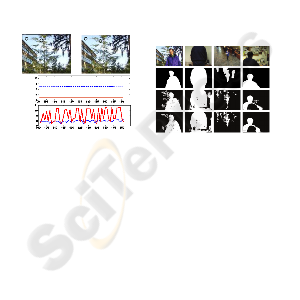
to remain labeled as FG. In Fig.2, an explicative com-
A
B
fr.
108
A
B
B
A
fr.
140
σ
(t)
A,r
hit
σ
(t)
B,r
hit
t
t
Figure 2: Evaluation of the standard deviation of the Gaus-
sian components of the TAPPMOG (blue-dashed line) and
S-TAPPMOG (red-solid line) models. Top: two frames
(108 and 140) of the WT sequence. Bottom: the frame evo-
lution of the standard deviations σ
(t)
r
hit
which characterize the
Gaussian components modeling the pixel signal related to
location A (top plot) and location B (bottom plot).
parison between TAPPMOG and our method is pro-
posed, where the parameters of TAPPMOG are the
same of the ones used in our method, except ρ
max
and
σ
max
, absent in TAPPMOG. Here, the standard devia-
tions of the Gaussian components that model the pixel
signals related to locations A and B are presented. For
ease the visualization, only the R channel is consid-
ered, and only the frame interval [100,150] is ana-
lyzed.
At frame 108, locations A and B are focused both
on the sky, but B depicts a zone more affected by
color variations, due to the tree presence. In the
two plots below the images, it can be noted that, at
frame 108, the standard deviation value assumed by
S-TAPPMOG is lower than the correspondent TAPP-
MOG value, highlighting the better precision with
which S-TAPPMOG models a wide and uniform as-
pect of the scene, i.e., the sky. At frame 140, location
A presents again the sky, while in location B the tree
is passing over. As a consequence, in the two plots
below, we can see that our method models the signal
representing the tree with higher standard deviation
as compared to the correspondent TAPPMOG value.
This indicates that S-TAPPMOG permits the tree of
assuming a larger spectra of signal values, thus di-
minishing the presence of false FG positives.
Qualitative results obtained by our method with the
WT sequence, together with the other dataset se-
quences and compared with the TAPPMOG method
are present in Fig.3. Note that the parametrization
chosen permits to TAPPMOG to obtain a better er-
ror rate than the one reported in ((Toyama et al.,
1999)) for the same sequences. Quantitative results,
WT C B FA
Figure 3: Wallflower qualitative results: on the first row, the
frames of the different sequences for which a ground truth is
provided; on the second row the ground truth; the third row
presents the TAPPMOG results and, finally, results obtained
with our method S-TAPPMOG are reported on the last row.
in terms of false positives (per-pixel false FG detec-
tions) and false negatives (missed FG detections) with
respect to other state of the art methods are visible
in Fig.4. In particular, Wallflower, SACON, Tracey
Lab LP, Bayesian Decision, and TAPPMOG refer to
((Wang and Suter, 2006; Kottow et al., 2004; Nakai,
1995; Stauffer and Grimson, 1999)), respectively,
which have been previously discussed in Sect.2. As
visible in Fig.4, our method outperforms globally
Wallflower, Bayesian decision and TAPPMOG meth-
ods, providing also good results with respect to Sacon
and Tracey Lab LP methods, which are however more
structured and time demanding techniques, tightly
constrained to initial hypotheses. Please note that we
did not report the good results reached in ((H. Wang,
2005)), because we are not convinced deeply about
the RGB normalized signal modeling proposed in that

7844
1912
377
2289
1414
811
2225
643
1382
2025
153
1152
1305
f.neg.
f.pos.
t.e.
STAPPMOG
10059
2217
870
3087
1732
1033
2765
220
2398
2618
56
1533
1589
f.neg.
f.pos.
t.e.
TAPPMOG
14043
2501
1974
4485
2143
2764
4907
1538
2130
3688
629
334
963
f.neg.
f.pos.
t.e.
Bayesian
decision
7219
2403
356
2759
1974
92
2066
1998
69
2067
191
136
327
f.neg.
f.pos.
t.e.
Tracey LAB
LP
4084
1508
521
2029
1150
125
1275
47
462
509
41
230
271
f.neg.
f.pos.
t.e.
SACON
9170
320
649
969
2025
365
2390
229
2706
2935
877
1999
2876
f.neg.
f.pos.
t.e.
Wallflower
T.Err.FABCWTErr.
Methods
Figure 4: Quantitative results obtained by the proposed S-
TAPPMOG method: f.neg,f.pos.,t.e.,and T.Err mean false
negative, false positive per-pixel FG detections, total errors
on the specific sequence and total errors summed on all
the sequences analyzed, respectively. Our method outper-
formed the most effective general purposes BG subtraction
scheme (Wallflower, Bayesian decision, TAPPMOG), and
is comparable with methods which are more time demand-
ing and strongly constrained by data-driven initial hypothe-
ses (SACON and Tracey Lab LP).
paper. There, the RGB-normalized signal covariance
matrix was modeled as a diagonal matrix, while this
fact is not correct, as mentioned in ((Mittal and Para-
gios, 2004)).
5.2 “Traffic” Dataset
This dataset is formed by outdoor traffic sequences.
We focus on two of them, the “Snow” and the “Fog”
sequences, which are characterized by very hard
weather conditions, see Fig.5, first row.
As comparison against our method, we apply the
TAPPMOG algorithm, choosing the following param-
eters set: α = 0.005, w
init
= 0.01, σ
init
= 7.5. With the
same parameters setting, we apply the S-TAPPMOG
algorithm with γ
max
= 20 and ρ
max
= 7. In order to
speed up the processing, we down-sample both the
sequences reducing them to 160 × 120 pixel frames,
obtaining performances of 8 frames per sec. with the
TAPPMOG method and 6 frames per sec. with the S-
TAPPMOG algorithm, with MATLAB not-optimized
code.
Some qualitative results are shown in Fig.5. In gen-
eral, TAPPMOG method produces a large amount
of false FG detections. The following considera-
tions explain this phenomenon. In the “Snow” se-
quence (please refer to Fig.5, first three columns),
the scene can be modeled by a bi-modal BG, i.e.,
one mode modeling the outdoor environment, and
the other modeling the snow. The snow generates a
high-variance color intensity pattern, which can be in-
tended as a spatial texture (i.e., a pattern which glob-
ally cover the scene). Modeling this texture by taking
into account for signals coming from different close
positions is equivalent to better capture the intrinsic
high variance of the appearance of the snow. As an
example, see the red false FG detections in the related
figures, which are globally fewer than in the TAPP-
MOG approach. In particular, in Fig.5a, the snow
causes more false FG detections in the center of the
scene with the TAPPMOG model.
At the same time, the other component modeling the
clean environment (not corrupted by the snow), can
be learnt more precisely (with a smaller standard de-
viation), refining the per-pixel signal estimation with
the neighboring similar pixels signals. Looking at
Fig.5b), one can note that the car on the bottom is
not discovered by TAPPMOG approach, whereas it is
partially detected by S-TAPPMOG. A similar obser-
vation can be assessed by observing the car on Fig.5c,
which is better modeled by S-TAPPMOG.
In any case, the per-region analysis of the S-
TAPPMOG brings a side effect: when a white ob-
ject passes over the scene, this can be absorbed by the
white large variance BG Gaussian component which
characterizes the snow, causing a FG miss. This is
visible in Fig.5a, where the first car from the top is
partially covered by the lamp on the upper left part of
the image and some gray part of the tram on Fig.5b
and Fig.5c.
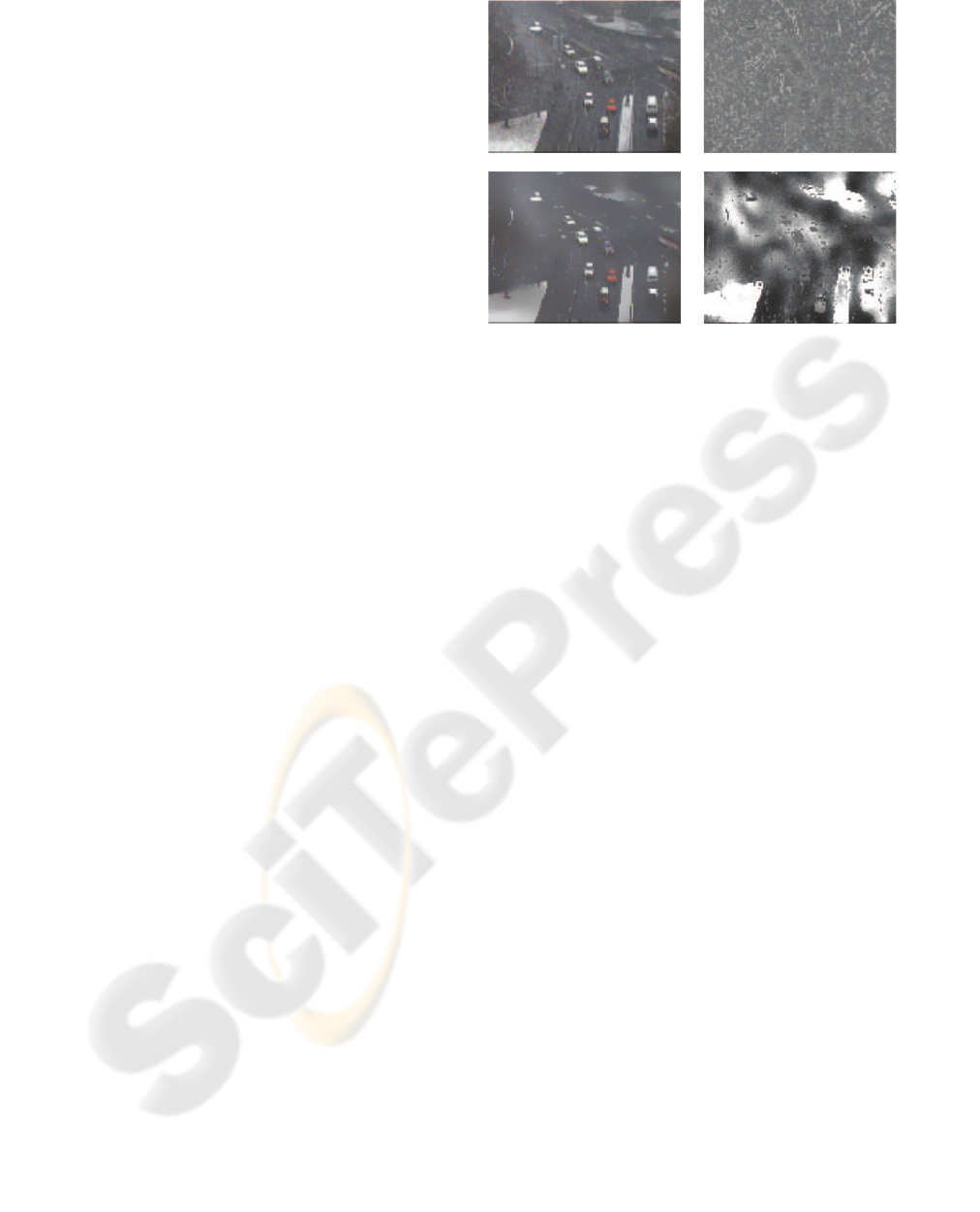
As visual explanation of how differently the two
methods model the scene, please refer to Fig.6. From
the images depicting the σ values, it is visible that our
method permits to better extract FG objects where the
scene is more uniform, e.g., the street, whereas in the
zones in which the scene can be confused with the
snow, standard deviation values are higher. As a com-
parison, in the corresponding images of the TAPP-
MOG method, no spatial distinction is made in the
FG discrimination, and, in general, the value of the
standard deviation is higher. From the µ images, in
S-TAPPMOG, we can see that the FG objects better
protrude with respect to the rest of the BG scene. This
means that the mean values that characterize FG and
BG objects are better differentiated by S-TAPPMOG
with respect to the TAPPMOG method. Similar con-
siderations can be stated for the “Fog” sequence (re-
fer to Fig.5, third column). Here, the scene can be
characterized by a bimodal BG, where one compo-
nent models the scene heavily occluded by the fog,
and the other explains the scene when the fog drasti-
cally diminishes, due to the characteristic dynamics of
the fog banks. In this case, the low-variance, per-pixel

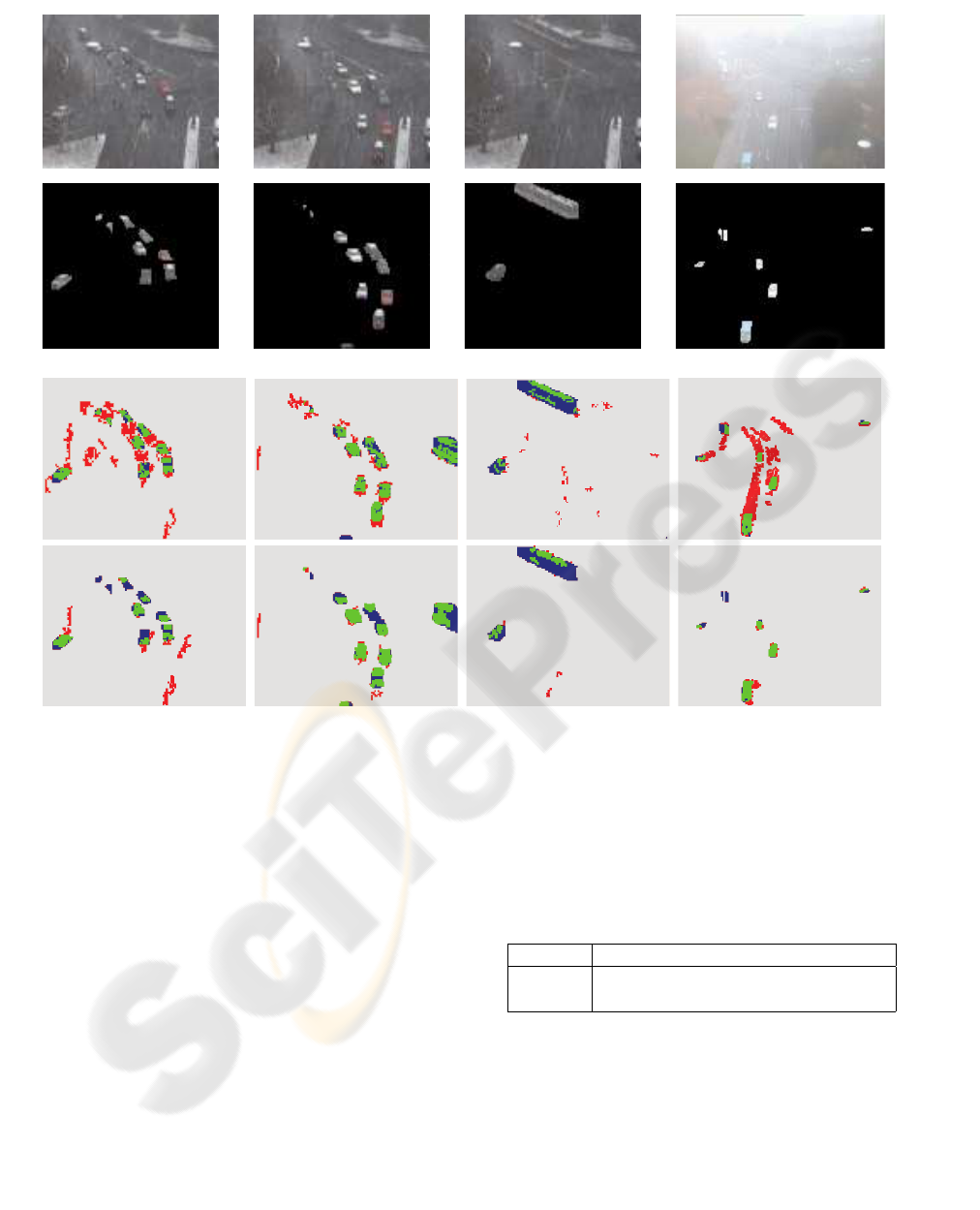
a) fr.34 b) fr.118 c) fr.284 d) fr.284
Figure 5: “Traffic” dataset results: three frames of the “Snow” sequence and one frame of the “Fog” sequence (first row);
hand-segmented ground truth (second row); TAPPMOG method (third row); our method (fourth row). In the two last rows
(the figure will be printed in color), green pixels mean correct FG detections, red pixels mean false FG detections (false
positives), and blue pixels mean undetected FG pixels (false negatives).
Gaussian components are not able to model sudden
local changes of fog intensity, while the S-TAPPMOG
model works better. Nevertheless, in some cases
white FG objects are more difficult to discover for S-
TAPPMOG than for the TAPPMOG method.
In order to test quantitatively the two algorithms,
we perform a manual counting operation for each
original frame of the two sequences, extracting the
number of separated objects moving on the scene.
For each frame we manually label with a mark the
center of each distinct moving object. Then, using
a connected components operator, we extract the FG
blobs from each output frame found by the two al-
gorithms. After that, we control if each blob inter-
sects one FG mark manually annotated. If a FG blob
does not intersect any mark, we annotate a false FG
Table 1: Accuracy test for the “Snow” and “Fog” sequences,
in terms of total errors.
Seq. TAPPMOG err. S-TAPPMOG err.
“Snow” 2253 1807
“Fog” 1501 845
detection and if a mark remains uncovered, we anno-
tate a FG miss. The summation of all false negatives
and false positives gives the total error rate, shown in
Tab.1. This test can give an idea on how our method
performs when embedded in a multi-object tracking
framework, where the separation of different objects
plays an important role in the data association. As
visible by the results, in both the cases the errors are

less for S-TAPPMOG. This, together with the analy-
sis done with the Wallflower dataset, demonstrates the
qualities of the proposed approach.
REFERENCES
H. Wang, D. S. (2005). A re-evaluation of mixture of gaus-
sian background modeling. In Proc. of the IEEE Int.
Conf. on Acoustics, Speech, and Signal Processing,
2005 (ICASSP ’05), volume 2, pages ii/1017– ii/1020.
Heikkila, M. and M.Pietikainen (2006). A texture-based
method for modeling the background and detecting
moving objects. IEEE Trans. Pattern Anal. Mach. In-
tell., 28(4):657–662.
Isard, M. and Blake, A. (1998). CONDENSATION: Con-
ditional density propagation for visual tracking. Int. J.
of Computer Vision, 29(1):5–28.
Kottow, D., K
¨
oppen, M., and del Solar, J. (2004). A back-
ground maintenance model in the spatial-range do-
main. In ECCV Workshop SMVP, pages 141–152.
Mittal, A. and Paragios, N. (2004). Motion-based back-
ground subtraction using adaptive kernel density esti-
mation. In CVPR ’04: Proceedings of the IEEE Com-
puter Society Conference on Computer Vision and
Pattern Recognition, pages 302–309. IEEE Computer
Society.
Nakai, H. (1995). Non-parameterized bayes decision
method for moving object detection. In Proc. Second
Asian Conf. Computer Vision, pages 447–451.
Noriega, P. and Bernier, O. (2006). Real time illumina-
tion invariant background subtraction using local ker-
nel histograms. In Proc. of the British Machine Vision
Conference.
Ohta, N. (2001). A statistical approach to background sub-
traction for surveillance systems. In Int. Conf. Com-
puter Vision, volume 2, pages 481–486.
Stauffer, C. and Grimson, W. (1999). Adaptive back-
ground mixture models for real-time tracking. In
Int. Conf. Computer Vision and Pattern Recognition
(CVPR ’99), volume 2, pages 246–252.
Stenger, B., nad N. Paragios, V. R., F.Coetzee, and Buh-
mann, J. M. (2001). Topology free hidden Markov
models: Application to background modeling. In Int.
Conf. Computer Vision, volume 1, pages 294–301.
Toyama, K., Krumm, J., Brumitt, B., and Meyers, B.
(1999). Wallflower: Principles and practice of back-
ground maintenance. In Int. Conf. Computer Vision,
pages 255–261.
Wang, H. and Suter, D. (2006). Background subtrac-
tion based on a robust consensus method. In ICPR
’06: Proceedings of the 18th International Confer-
ence on Pattern Recognition (ICPR’06), pages 223–
226, Washington, DC, USA. IEEE Computer Society.
Wren, C., Azarbayejani, A., Darrell, T., and Pentland, A.
(1997). Pfinder: Real-time tracking of the human
body. IEEE Transactions on Pattern Analysis and Ma-
chine Intelligence, 19(7):780–785.
µ
TAPPMOG
σ
TAPPMOG
µ
S-TAPPMOG
σ
S-TAPPMOG
Figure 6: Different modeling for the frame 118 of
the “Snow” sequence, performed by TAPPMOG and S-
TAPPMOG. In the µ images the mean value of the Gaussian
component modeling the signal is depicted for each pixel.
The same holds for the σ images, where brighter pixels cor-
respond to higher standard deviation values.