
EXTERIOR ORIENTATION USING LINE-BASED ROTATIONAL
MOTION ANALYSIS
A. Navarro, E. Villarraga and J. Aranda
Technical University of Catalonia, ESAII Department, Barcelona, Spain
Keywords: Exterior orientation, motion analysis, hand-eye calibration, pose estimation.
Abstract: 3D scene information obtained from a sequence of images is very useful in a variety of action-perception
applications. Most of them require perceptual orientation of specific objects to interact with their
environment. In the case of moving objects, the relation between changes in image features derived by 3D
transformations can be used to estimate its orientation with respect to a fixed camera. Our purpose is to
describe some properties of movement analysis over projected features of rigid objects represented by lines,
and introduce a line-based orientation estimation algorithm through rotational motion analysis.
Experimental results showed some advantages of this new algorithm such as simplicity and real-time
performance. This algorithm demonstrates that it is possible to estimate the orientation with only two
different rotations, having knowledge of the transformations applied to the object.
1 INTRODUCTION
Perceptual orientation of specific objects in a 3D
scene is necessary in a diversity of action-perception
applications where 2D information is the only input.
Automated navigation or manipulation are examples
of this kind of applications and rely heavily in 2D
data obtained from a video camera as sensory input
to fulfill 3D tasks. The exterior orientation problem
serves to map the 2D-3D relation estimating the
transformation between coordinate frames of objects
and the camera.
There are several methods proposed to estimate
the orientation of a rigid object. The first step of
their algorithms consists on the identification and
location of some kind of features that represent an
object in the image plane. Most of them rely on
feature points and apply closed-form or numerical
solutions depending on the number of objects and
image feature correspondences. Previous works
focused with a small number of correspondences
applied iterative numerical techniques as (Lowe,
1987) and (Haralick et al., 1991). Other methods
apply direct linear transform (DLT) for a larger
number of points as (Hartley, 1998) or reduce the
problem to close-form solutions, as (Fiore, 2001)
applying orthogonal decomposition.
Lines, however, are the features of interest in this
work. They are the features to be extracted from a
sequence of images and provide motion information
through its correspondences. There are several
approaches that use this kind of features to estimate
motion parameters. Some early works solve a set of
nonlinear equations, as the one by (Yen and Huang,
1983), or use iterated extended Kalman filters, as
showed by (Faugeras et al., 1987), through three
perspective views. Works by (Ansar and Daniilidis,
2003) combined sets of lines and points for a linear
estimation, and (Weng et al., 1992) discussed the
estimation of motion and structure parameters
studying the inherent stability of lines and explained
why two views are not sufficient.
An important property in using lines is their
angular invariance between them. Then, our purpose
was to study this property to provide a robust
method to solve orientation estimation problems. It
is possible to compute the orientation of an object
through the analysis of angular variations in the
image plane induced by its 3D rotations with respect
to the camera. It can be seen as an exterior
orientation problem where objects in the scene are
moved to calculate their pose.
Some action-perception applications can be seen
as a fixed camera visualizing objects to be
manipulated. In our case, these objects were
represented by lines. Three views after two different
rotations generate three lines in the image plane,
each of them define a 3D plane called the projection
plane of the line. These planes pass through the
290
Navarro A., Villarraga E. and Aranda J. (2007).
EXTERIOR ORIENTATION USING LINE-BASED ROTATIONAL MOTION ANALYSIS.
In Proceedings of the Second International Conference on Computer Vision Theory and Applications - IU/MTSV, pages 290-293
Copyright
c
SciTePress
P
a
P
b
P
c
Camera
frame
Image plane
Object
Centroid
Intersection line
Object
end point
R
1
R
2
P
a
P
b
P
c
Camera
frame
Image plane
Object
Centroid
Intersection line
Object
end point
R
1
R
2
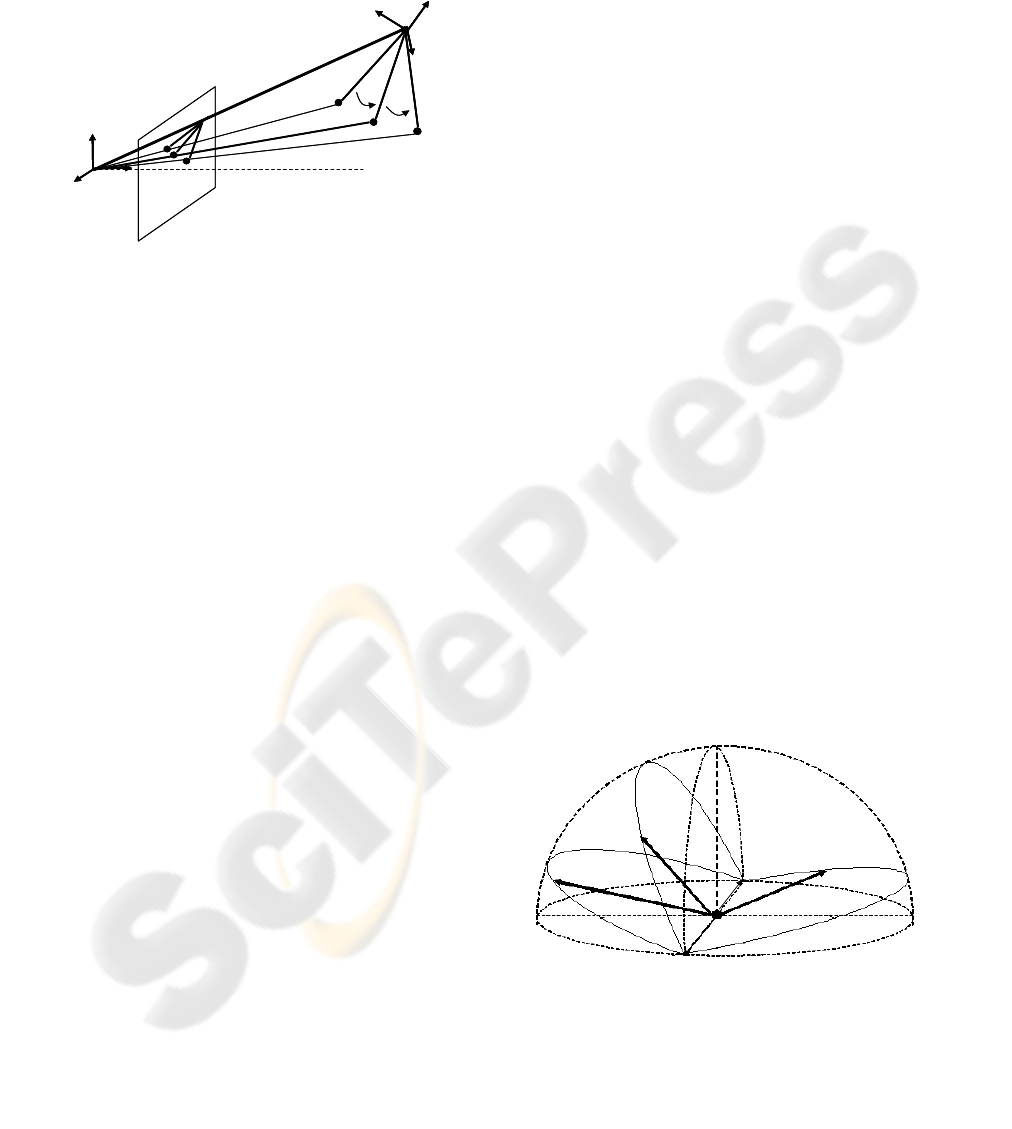
projection center and their respective lines. Their
intersection is a 3D line that passes through the
origin of the perspective camera frame and the
centroid of the rotated object, as seen in Figure 1.
The motion analysis of angular variations
between lines permitted us to estimate the
orientation of a given object. Therefore, we propose
a robust method to compute the orientation through
rotations. These rotations must be known. They
could be sensed or given and controlled, as is the
case of robotic applications. Experimental results
showed some advantages of this new algorithm such
as simplicity and real-time performance.
2 ORIENTATION ESTIMATION
ALGORITHM
Motion analysis of feature lines was the base of our
orientation estimation algorithm. In this case known
3D rotations of a line and its subsequent projections
in the image plane were related to compute its
relative orientation with respect to a perspective
camera. Vision problems as feature extraction and
line correspondences are not discussed and we
suppose the focal distance f as known. Our goal is,
having this image and motion information, estimate
the orientation of an object represented by feature
lines with the minimum number of movements and
identify patterns that permits to compute a unique
solution without defined initial conditions.
2.1 Mathematical Analysis
A 3D plane is the result of the projection of a line in
the image plane. It is called the projection plane and
passes through the projection center of the camera
and the 3D line. This 3D line, in this case, is the
representation of an object. With three views after
two different rotations of the object, three lines are
projected in the image plane. Thus three projection
planes can be calculated. These planes are P
a
, P
b
and
P
c
, and their intersection is a 3D line that passes
through the projection center and the centroid of the
rotated object, being the centroid the point of the
object where it is rotated. Across this line a unit
director vector v
d
can be determined easily knowing
f and the intersection point of the projected lines in
the image plane. Our intention is to use this 2D
information to formulate angle relations with the 3D
motion data.
Working in the 3D space permits to take
advantage of the motion data. In this case where the
object is represented by a 3D line, the problem could
be seen as a unit vector across its direction that is
rotated two times. In each position of the three views
this unit vector lies in one of the projection planes as
seen in Figure 2. It first is located in P
a
, then it
rotates an angle α
1
to lie in P
b
and ends in P
c
after
the second rotation by an angle α
2
. To estimate the
relative orientation of the object we first must obtain
the location of three unit vectors, v
a,
v
b
and v
c
, that
coincide with the 3D motion data and lie on their
respective planes. To do this we know that the scalar
product of:
1
.cos
ab
vv
α
=
(1)
2
.cos
bc
vv
α
=
(2)
Calculating the angle γ between the planes formed
by v
a
v
b
and v
b
v
c
from the motion information, we
have
(
)
(
)
cos
ab bc
vvvv
γ
××= (3)
And applying vector identities
12
. cos cos cos
ac
vv
α
αγ
=
− (4)
With the set of equations conformed by (1), (2)
and (4) we have the three unit vectors to calculate.
Figure 1: A 3D line through the origins is the intersection
of the projection planes after two rotations of the object.
P
a
P
b
P
c
v
a
v
b
v
c
v
d
P
a
P
b
P
c
v
a
v
b
v
c
v
d
Figure 2: Unit vectors Va, Vb and Vc are constrained to lie
on planes Pa, Pb and Pc respectively. Their estimation can
be seen as a semi sphere where their combination must
satisfy the angle variations condition.
EXTERIOR ORIENTATION USING LINE-BASED ROTATIONAL MOTION ANALYSIS
291

However, there is not a unique solution, thus
constraints must be applied.
2.2 Projection Planes Constraint
There are many possible locations where the three
unit vectors can satisfy the equations in the 3D
space. To obtain a unique solution unit vectors v
a
, v
b
and v
c
must be constrained to lie in their respective
planes. Unit vector v
a
could be seen as any unit
vector in the plane P
a
rotated through an axis and an
angle. Using unit quaternions to express v
a
we have
*
aaa
vqvq= (5)
where q
a
is the unit quaternion applied to v
a
, q
a
*
is its conjugate and v is any vector in the plane. For
every rotation about an axis n, of unit length, and
angle Ω, a corresponding unit quaternion q = (cos
Ω/2, sin Ω/2 n) exists. Thus v
a
is expressed as a
rotation of v, about an axis and an angle by unit
quaternions multiplications. In this case n must be
normal to the plane P
a
if both unit vectors v
a
and v
are restricted to be in the plane.
Applying the plane constraints and expressing v
a
,
v
b
and v
c
as mapped vectors through unit
quaternions, equations (1), (2) and (4) can be
expressed as a set of three nonlinear equations with
three unknowns
**
1
cos
ad a bd b
qvqqvq
α
=
(6)
**
2
cos
bd b cd c
qvqqvq
α
= (7)
**
12
cos cos cos
ad a cd c
qvqqvq
α
αγ
=− (8)
The vector to be rotated is v
d
, which is common to
the three planes, and their respective normal vectors
are the axes of rotation. Extending the equations (6),
(7) and (8), multiplying vectors and quaternions,
permits to see that there are only three unknowns
which are the angles of rotation Ω
a
, Ω
b
and Ω
c
.
Applying iterative numerical methods to solve
the set of nonlinear equations, the location of v
a
, v
b
and v
c
with respect to the camera frame in the 3D
space are calculated. Now we have a simple 3D
orientation problem that can be solved easily by a
variety of methods as least square based techniques.
However, in the case where motions could be
controlled and selected movements applied, this last
step to estimate the relative orientation would be
eliminated. Rotation information would be obtained
directly from the numerical solution. If we assume
one of the coordinate axes of the object frame
coincide with the moving unit vector and apply
selected motions, as one component rotations, a
unique solution is provided faster and easier.
3 EXPERIMENTAL RESULTS
Real world data was used to validate the algorithm.
Experiments were carried out through a robotic test
bed that was developed in order to get high
repeatability. It consist on an articulated robotic arm
with a calibrated tool frame equipped with a tool,
easily described by a line, which is presented in
different precisely known orientations to a camera.
The camera field of view remains fixed during the
image acquisition sequence. The tool center of
rotation is programmed to be out of the field of
view, as it would be presented in an action-
perception application.
With this premises, an standard analog B/W
camera equipped with a known focal lenght optics
has been used. This generates a wide field of view
that is sampled at 768x576 pixels resolution. After
image edge detection, Hough Transform is used in
order to obtain the tool contourn and the straight line
in the image plane associated to it. Tool contourn is
supossed to have the longest number of aligned pixel
edges in the image.
Having this setup, feature lines were identified
and located in a sequence of images. This images
captured selected positions of the rotated tool. Once
the equation of the lines projected in the image plane
were acquired, unit vectors normal to the constraint
planes and v
d
could be calculated. This unit vectors
and the motion angles α
1
and α
2
served as the input
to the proposed algorithm. The intersection of the
lines was needed to calculate v
d
. This calculation is
prone to errors due to be located out of the field of
view. It means the intersection of a different number
of lines is not usually the same point. Table 1 shows
the standard deviation in pixels of the intersection
points calculated through different motion angles.
The intersections converge to a single point when
the angles between lines are higher.
Table 1: Standard deviation of intersecting lines (in pixels)
through different motion angles. Being the intersection
point defined by Xint and Yint.
Degrees Xint Yint σ
5
895,81 264,11 62,31
10
928,28 278,91 35,65
15
861,41 250,71 6,958
20
876,67 256,52 5,83
The 3D transformation resultant from the algorithm
was tested projecting 3D lines, derived by new tool
rotations, in the image plane and comparing them
with the line detected by the vision system. Tests for
motion angles between 5 and 20 degrees were
VISAPP 2007 - International Conference on Computer Vision Theory and Applications
292
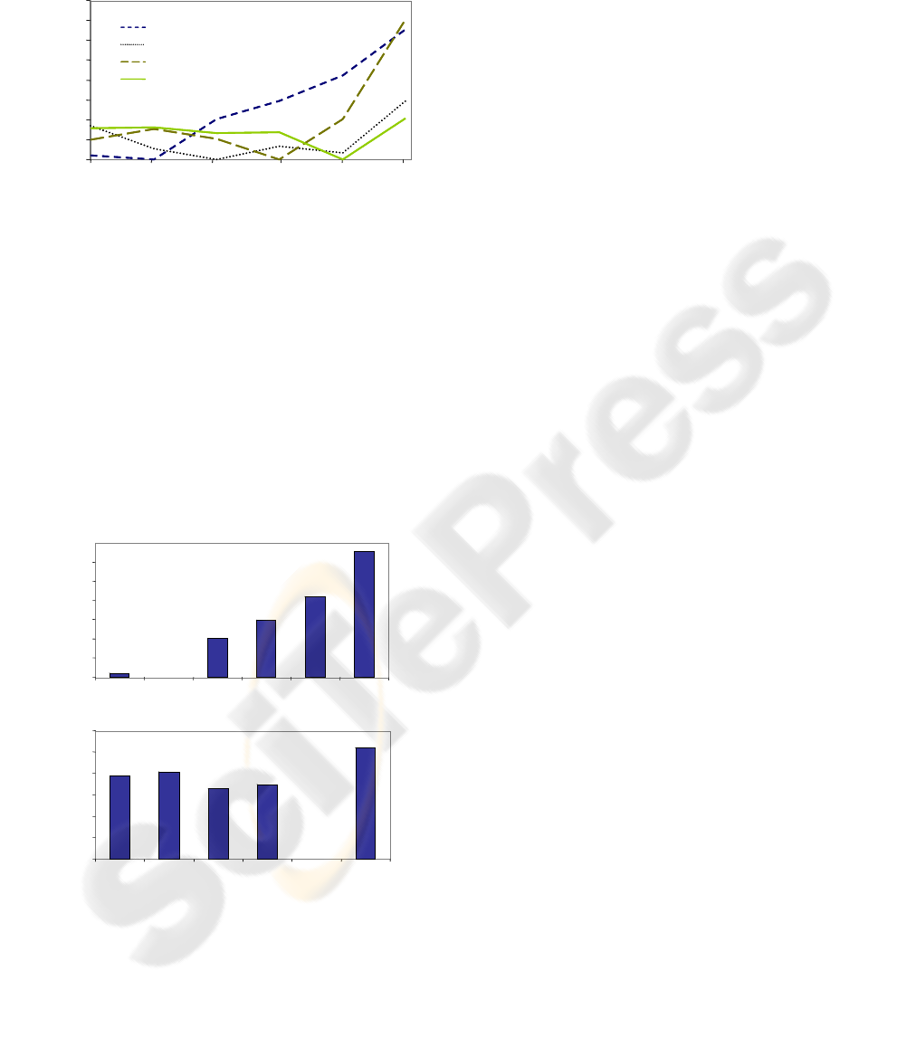
carried out. Figure 3 shows the error (in pixels)
between lines through different angles.
There can be seen how the error is minimum at
the position where the transformation was
calculated, it means at its second motion or third
image. This error varies depending on the position of
the tool, it increases with higher angles, when the
position of the tool separates from the minimum
error position. Figure 4 compares the algorithm
performance for 5 and 20 degrees motion angles.
There the error varies differently. In the case of 5
degrees the error increases greatly with each motion
that separates the tool from the minimum error
position. While for 20 degrees this error also
increments, but remains stable.
This results validate the line-based algorithm and its
low computational cost demonstrate its real-time
performance. The error increasement with large
position separations is mainly product of the
deviation at the intersection point. It can be seen that
the calculation of vd has a great impact in the result
and future work should be focused in this issue.
4 CONCLUSIONS
A method to estimate the relative orientation of an
object with respect to a camera has been proposed.
The object assumed was represented by feature
lines. 2D correspondences of a line due to known 3D
transformations of the object were the information
used to calculate its orientation. We showed that
with only two rotations the angular variation
between lines provides sufficient information to
estimate the relative orientation. This motion
analysis led to address questions as the uniqueness
of solution for the minimum number of movements
and possible motion patterns to solve it directly. In
the case of controlled motions, one component
rotations through normal axes simplify calculations
to provide a robust technique to estimate the relative
orientation with no initial conditions defined.
REFERENCES
Ansar, A., Daniilidis, K., 2003. Linear pose estimation
from points and lines. In IEEE Trans. Pattern Analysis
and Machine Intelligence. 25:578-589.
Faugeras, O., Lustran F., Toscani G., 1987. Motion and
structure from point and line matches. In Proc. First
Int. Conf. Computer Vision.
Fiore, P., 2001. Efficient linear solution of exterior
orientation. In IEEE Trans. Pattern Analysis and
Machine Intelligence. Vol 23, No 2.
Haralick, R.M., Lee, C., Ottenberg, K., Nölle, M., 1991.
Analysis and solutions of the three point perspective
pose estimation problem. In IEEE Conf. Computer
Vision and Pattern Recognition.
Hartley, R.I., 1998. Minimizing algebraic error in
geometric estimation problems. In Proc. Int. Conf.
Computer Vision (ICCV), pp. 469-476.
Lowe, D.G., 1987. Three-dimensional object recognition
from single two-dimensional images. In Artificial
Intelligence, vol. 31, no. 3, pp.
Weng, J., Huang, T.S., Ahuja, N., 1992. Motion and
structure from line correspondences; closed-form
solution, uniqueness, and optimization. In IEEE Trans.
Pattern Analysis and Machine Intelligence. Vol. 14,
3:318-336.
Yen B.L., Huang T.S., 1983. Determining 3-D motion and
structure of a rigid body using straight line
correspondences. In Image sequence Processing and
Dynamic Scene Analysis, Heidelberg, Germany:
Springer-Verlag.
0
10
20
30
40
510152025
5º
10º
15º
20º
Angles α1, α2 (degrees)
Relative error (pixels)
Orientation error
0
10
20
30
40
510152025
5º
10º
15º
20º
Angles α1, α2 (degrees)
Relative error (pixels)
Orientation error
Figure 3: Relative error in pixels using the rotational
motion analysis algorithm.
0
10
20
30
0 5 10 15 20 25
Orientation error increment for 5 degrees motion angle
Angles α1+ α2 (degrees)
Relative error (pixels)
0
10
20
30
0 5 10 15 20 25
Orientation error increment for 5 degrees motion angle
Angles α1+ α2 (degrees)
Relative error (pixels)
0
4
8
12
0 5 10 15 20 25
Orientation error increment for 20 degrees motion angle
Relative error (pixels)
Angles α1+ α2 (degrees)
0
4
8
12
0 5 10 15 20 25
Orientation error increment for 20 degrees motion angle
Relative error (pixels)
Angles α1+ α2 (degrees)
Figure 4: Algorithm performance comparation between 5
and 20 degrees, with a first rotation α1 followed by
a
second α2 of the same magnitude.
EXTERIOR ORIENTATION USING LINE-BASED ROTATIONAL MOTION ANALYSIS
293
