METHODS USED IN INCREASED RESOLUTION PROCESSING

Polygon Based Interpolation and Robust Log-polar Based Registration

Stéfan van der Walt and Ben Herbst

University of Stellenbosch, South Africa

Keywords:

Geometry, interpolation, registration, image-processing, astronomy, log-polar transform.

Abstract:

A polygon-based interpolation algorithm is presented for use in stacking RAW CCD images. The algorithm

improves on linear interpolation in this scenario by closely describing the underlying geometry. 25 frames

are stacked in a comparison. When stacking images, it is required that these images are accurately aligned.

We present a novel implementation of the log-polar transform that overcomes its prohibitively expensive com-

putation, resulting in fast, robust image registration. This is demonstrated by registering and stacking CCD

frames of stars taken by a telescope.

1 INTRODUCTION

In this paper we describe two techniques which have

proved useful in the construction of resolution reﬁn-

ing algorithms. The ﬁrst is polygon-based interpola-

tion. When stacking RAW CCD readouts, the frames

are aligned and interpolation is applied to obtain val-

ues on a common grid. Unlike bi-linear interpola-

tion, that can cause blur and is not well suited to the

geometry of the problem, geometric interpolation is

designed to take not only the positions but also the

shape of pixels into account.

The second technique is image registration or

alignment using the log-polar transform (LPT). While

the LPT has been proposed for this purpose before,

the computational cost is prohibitive. We show how

the LPT can beused in a way that requires much fewer

computations, without compromising robustness or

accuracy.

2 POLYGON-BASED

INTERPOLATION

Given an image, or grid of pixel values, we would like

to calculate the value at an arbitrary point in the grid.

Bi-linear interpolation esentially uses a weighted av-

erage of the closest four pixels, based on their dis-

tances from the target position (Press et al., 2003). If

pixels are seen as inﬁnitely small points in space, this

method yields accurate results.

When, however,weconsider that pixelshaveﬁnite

areas, this method is only reasonably accurate when

the target pixel is horizontally and vertically aligned

with the original grid. As soon as rotation or skew

comes into play, linear interpolation no longer resem-

bles the underlying geometry, as is the case when

stacking raw CCD frames. The CCD sensor com-

prises a number of light-sensitivecapacitors, arranged

in a grid. For the purpose of this article we will as-

sume that the shape of these capacitors is square, but

the method described allows for any geometry, also

in the arrangement on the sensor itself (permitted that

there are no holes, as in the case of the colour-masked

CCD).

Given a target pixel position, (r,s), and a trans-

formed (for example rotated and translated) source

pixel at (m,n) with value W

m,n

, we would like to cal-

culate the contribution of the source to the target. We

construct a quadrilateral polygon at the target position

with vertices



s s+ 1 s+ 1 s

r r r+ 1 r+ 1



135

van der Walt S. and Herbst B. (2007).

METHODS USED IN INCREASED RESOLUTION PROCESSING - Polygon Based Interpolation and Robust Log-polar Based Registration.

In Proceedings of the Second International Conference on Computer Vision Theory and Applications - IFP/IA, pages 135-140

 SciTePress

as well as at the reference position with vertices



n n+ 1 n+ 1 n

m m m+ 1 m+ 1



The vertices x

and y

are then inversely trans-

formed to align with the target grid. The source pixel

value is weighted with the area of the polygon inter-

section between source and target pixels (see Fig.1).

This method has the advantage that it can be adapted

accurately for any kind of spatial transformation, al-

though it may require adding more vertices to support

non-linear transformations.

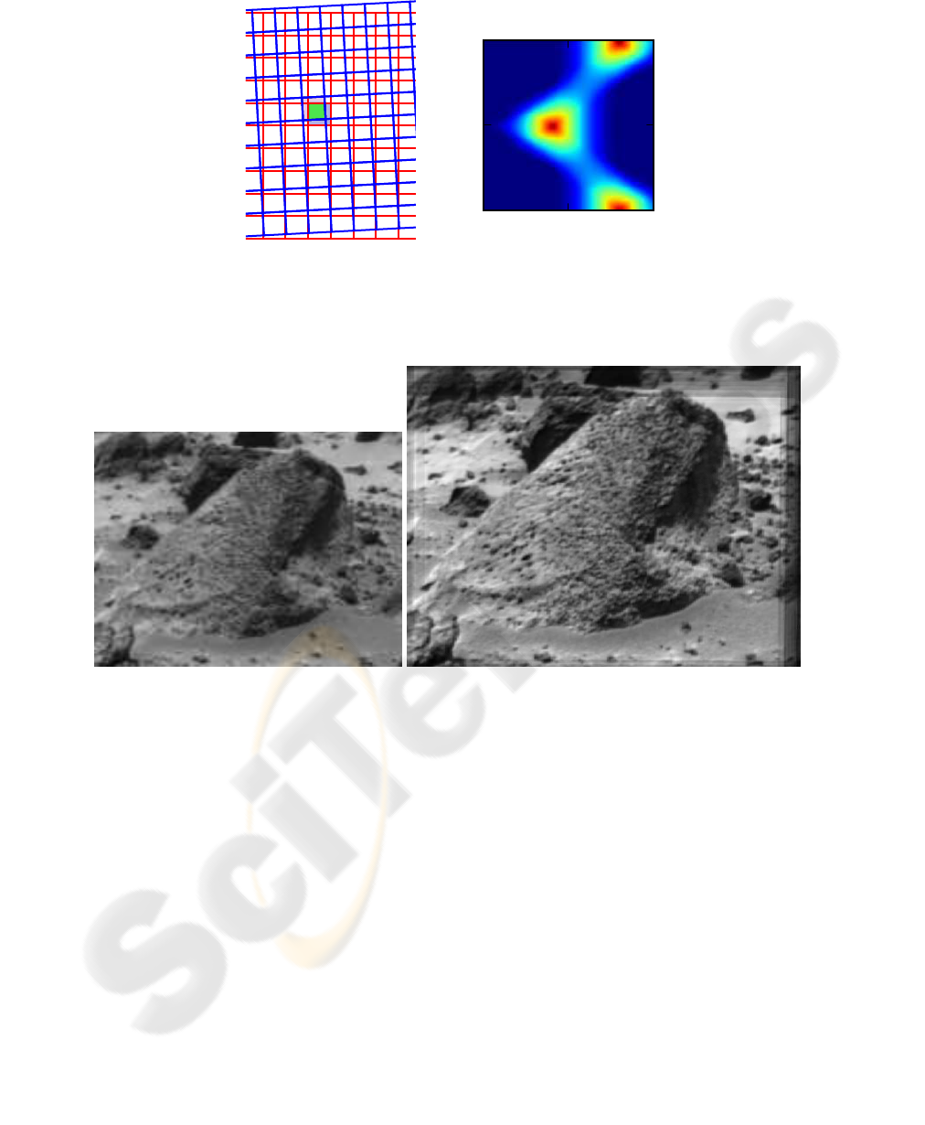
Using this technique, 25 frames provided by

the NASA Pathﬁnder mission were stacked (Peter

Cheeseman and Bob Kanefsky and Richard Kraft and

John Stutz and Robin Hanson, 1996). The frames

were aligned using localised features (Jianbo Shi

and Carlo Tomasi, 1994), with trivial outlier rejec-

tion. A high-resolution grid was speciﬁed after which

the polygon intersections were calculated using the

Liang-Barsky algorithm (You-Dong Liang and Brian

A. Barsky, 1983). The results are shown in Fig. 2.

Note that this is not a super-resolution algorithm (al-

though the interpolation can certainly be combined

with such a statistical estimation process), but simply

increased resolution stacking.

3 REGISTRATION

Registration algorithms can be divided into two broad

classes: those that operate in the spatial and fre-

quency (i.e. Fourier) domains, respectively. In the

spatial domain, there are sparse methods including

local descriptors, that depend on some form of fea-

ture extraction, and dense methods that operate di-

rectly on image values such as optical ﬂow and corre-

lation. The two classes generally differ in that the spa-

tial methods are localised, whereas the frequency do-

main methods (Reddy and Chatterji, 1996; Hanzhou

Liu and Baolong Guo and Zongzhe Feng, 2006; Has-

san Faroosh (Shekarforoush) and Josiane B. Zerubia,

2002; Harold S Stone and Stephen A Martucci and

Michael T Orchard and Ee-chien Chang, 2001) op-

erate globally. Attempts have been made to bridge

this gap, by using wavelet and other transforms to

locate information-carrying energy (George Lazardis

and Maria Petrou, 2006). These have been met with

varying success.

Each registration method has its own particu-

lar advantages and disadvantages. Fourier methods,

for example, are fast but inaccurate, suffer from re-

sampling and occlusion effects (Siavash Zokai and

George Wolberg, 2005, p. 1425), and only operate

globally. Iterative registration, on the other hand, is

highly accurate but extremely slow, and prone to mis-

registration due to local minima in the minimisation

space.

These problems led to the development of meth-

ods based on localised interest points (Carlo Tomasi

and Takeo Kanade, 1991; Jianbo Shi and Carlo

Tomasi, 1994; Tommasini et al., 1998; Tony Linde-

berg, 1998), such as the scale-invariant feature trans-

form (SIFT) (Lowe, 2003), the fast Speeded Up Ro-

bust Features (SURF) (Herbert Bay and Tinne Tuyte-

laars and Luc Van Gool, 2006) and others (K. Miko-

lajczyk and C. Schmid, 2002). All these methods de-

pend on unique localised features, which are available

in many images. There are, however, cases where it is

very difﬁcult to distinguish one feature from another

without examining its spatial context.

As an example, we will use frames recorded by a

CCD mounted on a telescope pointing at a deep-space

object. It is very difﬁcult to ﬁnd features to track in

these images, because the stars (all potential features)

are virtually identical and rotationally invariant. Since

local features fail, and global methods are slow and

unreliable, we would like to ﬁnd an algorithm that can

bridge the gap.

We will proceed to show that the log-polar trans-

form (LPT) is an ideal candidate. While previously

its use has been limited due to its high computational

cost, we develop ways of reducing those costs and

making the LPT behave more like local features.

4 THE LOG POLAR

TRANSFORM

The log-polar transform (LPT) spatially warps an im-

age onto new axes, angle (θ) and log-distance (L).

Pixel coordinates (x,y) are written in terms of their

offset from the centre, (x

), as

¯x = x− x

¯y = y− y

For each pixel, the angle is deﬁned by

θ =

(

arctan



¯y

¯x



¯x 6= 0

0 ¯x = 0

with a distance of

L = log



¯x

+ ¯y



The base, b, which determines the width of the trans-

form output, is chosen to be

b = e

ln(d)/w

= d

-1

0.25 1.5

Offset

−π

Angle

Figure 1: Illustration of the relation between interpolation weight and polygon overlap. A single polygon was transformed

with the given offset and angle to obtain the shown overlap, where blue represents zero and red represents one. Note that,

unlike with linear interpolation, the weights not only depend only on the distances between points.

(a) Sample input frame 1 (b) Polygon-based interpolation

Figure 2: Enhanced resolution obtained by stacking 25 frames, using polygon-based interpolation.

where d is the distance from (x

) to the corner of

the image, and w is the width or height of the input

image, whichever is largest.

When warping images, it is not possible to use the

forward transform. Since we use discrete coordinates

(integer x and y values), more than one input coordi-

nate may map to the same output coordinate. Worse

still, not every output coordinate will be covered.

One solution is to calculate the irregular grid of

coordinates obtained by transforming each input co-

ordinate (without discretising). Then, the input is

warped and resampled (using interpolation) at the re-

quired output positions. An easier and computation-

ally less intensive method is to reverse the process.

For each output coordinate, the transformation is ap-

plied in reverse, to obtain a coordinate in the input

image. Using interpolation, an output value is deter-

mined from the input. This can be done if, ignoring

the effect of discretisation, the transformation func-

tion is a one-to-one correspondence, and all input and

output coordinates are mapped.

Given θ and L , we would now like to ﬁnd x and y.

First, calculate the distance r from the centre,

r = e

ln(b)L

= e

Lln(d)/w

after which x and y can be recovered as

x = rcos(θ) + x

y = rsin(θ) + y

Note the relationship of the input image to the axes of

the LPT: if the input is rotated it results in a shift in

the θ axis, whereas scaling the input is seen as a shift

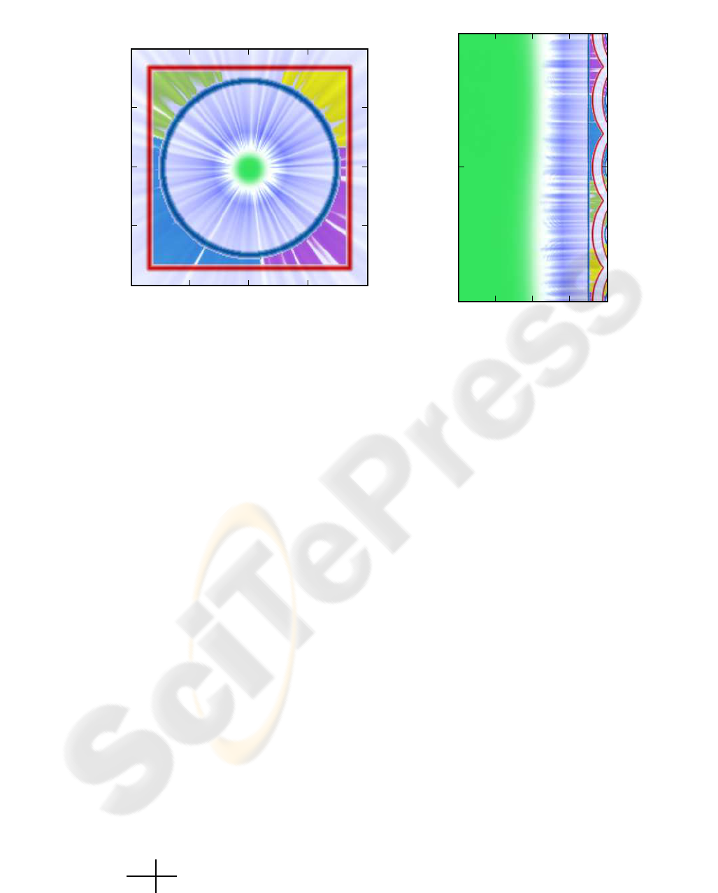
0 50 100 150 200

100

150

200

Colour input

1.00 3.45 11.89 41.01 141.42

Distance from centre

2π

Angle (θ)

Log polar transform

Figure 3: Illustration of the log-polar transform.

in the L axis. It is this property of the LPT that is used

in registration.

5 FAST REGISTRATION BASED

ON THE LOG-POLAR

TRANSFORM

In (Siavash Zokai and George Wolberg, 2005), afﬁne

registration based on the log-polar transform is de-

scribed. Given a reference frame, R(x,y), and a target

frame, B(x,y), we want to ﬁnd a transformation, T,

such that

R(x,y) = B(T(x,y)).

Assuming that the frames are images taken of the

same object from a long distance, we know that the

transformation must be a similarity, i.e. it is limited to

translation, rotation and scale. If we express a coordi-

nate (x,y) as a homogenous coordinate p = [x,y,1]

we can view the transformation as a matrix multipli-

cation,

T(p) = Mp

where

M =





scos(θ) −ssin(θ) t

ssin(θ) scos(θ) t

0 0 1









and R represents rotation, t translation and s scale.

The LPT proceeds as follows:

• From the centre of the reference frame, p

]

, cut a disc with a radius of roughly 20%

of the image width (larger or equal to the size of

the features we wish to track), and obtain its LPT.

• For each position in the target frame, p

= [x

]

cut out a disc of the same size as the reference

disc and obtain its LPT. Correlate the result with

the reference disc, taking care to wrap the angles-

axis. This is easily accomplished using the FFT.

If the normalised correlation is higher than at any

other point thus far, store the position, rotation (θ)

and scale (s).

The s and R components of M can now be determined,

after which the position is related to translation by

t = p

− sRp

The method outlined above is extremely robust, even

in the presence of high levels of noise, changes in il-

lumination and large differences in scale, rotation and

translation. Unfortunately, its computational com-

plexity proves to be prohibitive: even for a small

image of dimension 200 × 200, roughly 40000 log-

polar transforms and correlations need to be calcu-

lated. Furthermore, unless the target frame overlaps

with the centre of the reference frame, the registration

fails.

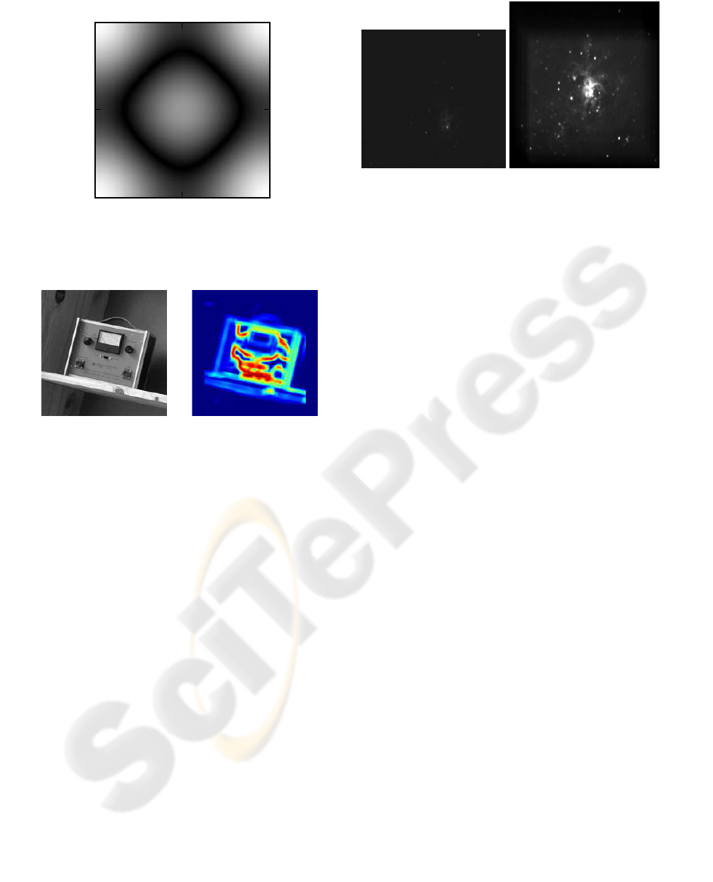
-1 0 1

-1

Figure 4: Fourier domain representation of the high-

frequency emphasis kernel.

Figure 5: The variance map highlights areas of interest.

To address this problem, we choose more discs in

the reference frame, but severely limit the number of

discs in the target frame, thereby reducing the number

of log-polar transforms and correlations that need to

be calculated. To accomplish this, we need to iden-

tify areas in both the reference and target frames that

are likely to contain useful features. Smooth areas are

less likely to contain such information. An intuitive

measure of smoothness is variance—as is often used

in texture analysis—but this commonly fails. For

example, imagine two images, one being a checker-

board pattern and the other divided in two halves, one

black and one white. The intensities in these images

will have the same variance, while their content and

texture differs. To counter this problem, we ﬁrst apply

the high-frequency emphasis kernel,

κ =





0 1 0

1 −1 1

0 1 0





of which the frequency response is shown in Figure 4,

to each frame. The variance is then calculated over a

moving window, yielding a map indicating potentially

useful features, as shown in Figure5.

(a) Example input frame (b) Result

Figure 6: Stacking is often used in astronomy to limit noise

and gather more light on the camera sensor. Here, 25 obser-

vations are stacked after automatic registration, using the

log-polar algorithm (photographs by Chris Forder of the

Cederberg Observatory).

To locate the position of such features, the map

is divided into smaller blocks, and the peak value in

each block is taken as the position of a disc. We use

16 equally-sized blocks in the reference frame and 40

equally-sized blocks in each of the target frames. Po-

sitions are rejected when the variance falls outside the

range of variances at reference positions. Discs can

also be rejected in terms of other criteria, for exam-

ple on the grounds of being symmetric, since such

discs can yield invalid matches at different angles.

The process outlined earlier is then followed, correlat-

ing discs in the reference and target frames to ﬁnd the

registration parameters. Note that the number of log-

polar transforms and correlations are reduced from

tens-of-thousands to fewer than 160. All log-polar

transforms use the same set of transformation coor-

dinates, which only need to be calculated once.

Since the variance map has a smoothing effect on

the input, we have to allow for a small error in the po-

sition of maximum correlation. A small search area,

typically 5× 5 pixels, is deﬁned around this point, for

which the registration is repeated to provide a reﬁned

measurement.

It is suggested in (Siavash Zokai and George Wol-

berg, 2005) that iterative minimisation of the registra-

tion parameters is performed, thereby increasing the

accuracy even further. We have found, however, that

this process often diverges due to the large number of

local minima in the minimisation space.

Figure 6 shows 25 frames from a telescope CCD

registered and stacked.

6 CONCLUSION

Linear interpolation is not equally well suited to all

applications. We show that an algorithm that is

closely related to the underlying geometry of an ap-

plication can yield results with higher accuracy.

For most applications in registration, localised in-

terest points provide fast, localised and accurate re-

sults. However, there are cases where these algo-

rithms fail, thus requiring a more robust algorithm.

The log-polar transform provides such an algorithm,

at signiﬁcant computational cost. Using the meth-

ods described in this paper, the computational cost

of LPT-based registration can be decreased, making

it both practical and effective.

REFERENCES

Carlo Tomasi and Takeo Kanade (1991). Detection and

Tracking of Point Features. Technical Report CMU-

CS-91-132, Carnegie Mellon University.

George Lazardis and Maria Petrou (2006). Image Registra-

tion Using the Walsh Transform. IEEE Transactions

on Image Processing, 15(8):2343–2357.

Hanzhou Liu and Baolong Guo and Zongzhe Feng (2006).

Pseudo-Log-Polar Fourier Transform for Image Reg-

istration. IEEE Signal Processing Letters, 13(1):17–

20.

Harold S Stone and Stephen A Martucci and Michael T

Orchard and Ee-chien Chang (2001). A fast direct

Fourier-based algorithm for subpixel registration of

images. IEEE Transactions on Geoscience and Re-

mote Sensing, 39(10):2235–2243.

Hassan Faroosh (Shekarforoush) and Josiane B. Zerubia

(2002). Extension of Phase Correlation to Subpixel

Registration. IEEE Transactions on Image Process-

ing, 11(3):188–200.

Herbert Bay and Tinne Tuytelaars and Luc Van Gool

(2006). SURF: Speeded Up Robust Features. In Pro-

ceedings of the ninth European Conference on Com-

puter Vision.

Jianbo Shi and Carlo Tomasi (1994). Good Features to

Track. In IEEE Conference on Computer Vision and

Pattern Recognition, pages 593–600.

K. Mikolajczyk and C. Schmid (2002). An Afﬁne Invariant

Interest Point Detector. In ECCV 1, number 128–142.

Lowe, D. (2003). Distinctive image features from scale-

invariant keypoints. International Journal of Com-

puter Vision, 20:91–110.

Peter Cheeseman and Bob Kanefsky and Richard Kraft and

John Stutz and Robin Hanson (1996). Super-Resolved

Surface Reconstruction from Multiple Images. In

Glenn R. Heidbreder, editor, Maximum Entropy and

Bayesian Methods. Kluwer Academic Publishers.

Press, W. H., Teukolsky, S. A., Vetterling, W. T., and Flan-

nery, B. P. (2003). Numerical Recipes in C++: The

Art of Scientiﬁc Computing. Cambridge University

Press, 2nd edition.

Reddy, B. and Chatterji, B. (1996). An FFT-based tech-

nique for translation, rotation, and scale-invariant

image registration. IEEE Transactions on Image

Processing, 5(8):1266–1271.

Siavash Zokai and George Wolberg (2005). Image Reg-

istration Using Log-Polar Mappings for Recovery

of Large-Scale Similarity and Projective Transfor-

mations. IEEE Transactions on Image Processing,

14(10):1422–1434.

Tommasini, T., Fusiello, A., Trucco, E., and Roberto, V.

(1998). Making good features track better. In Pro-

ceedings of the IEEE Conference on Computer Vision

and Pattern Recognition, pages 178–183, Santa Bar-

bara, CA. IEEE Computer Society Press.

Tony Lindeberg (1998). Feature Detection with Automatic

Scale Selection. International Journal of Computer

Vision, 30(2):77–116.

You-Dong Liang and Brian A. Barsky (1983). An analysis

and algorithm for polygon clipping. Communications

of the ACM, 26(11):868–877.