
RECONSTRUCTING IVUS IMAGES FOR AN ACCURATE TISSUE
CLASSIFICATION
Karla L Caballero, Joel Barajas
Computer Vision Center, Autonomous University of Barcelona, Edificio O Campus UAB, Bellaterra, Spain
Oriol Pujol
Dept. Matem
`
atica Aplicada i An
`
alisi. University of Barcelona, Computer Vision Center, Barcelona, Spain
Josefina Mauri
Hospital Universitari German Trias i Pujol, Badalona, Spain
Petia Radeva
Computer Vision Center, Autonomous University of Barcelona, Bellaterra, Spain
Keywords:
Intravascular Ultrasound, RF signals, Image Reconstruction, Tissue Classification, Adaboost, ECOC.
Abstract:
Plaque rupture in coronary vessels is one of the principal causes of sudden death in western societies. Reliable
diagnostic tools are of great interest for physicians in order to detect and quantify vulnerable plaque in order
to develop an effective treatment. To achieve this, a tissue classification must be performed. Intravascular
Ultrasound (IVUS) represents a powerful technique to explore the vessel walls and to observe its morphology
and histological properties. In this paper, we propose a method to reconstruct IVUS images from the raw
Radio Frequency (RF) data coming from the ultrasound catheter. This framework offers a normalization
scheme to compare accurately different patient studies. Then, an automatic tissue classification based on the
texture analysis of these images and the use of Adapting Boosting (AdaBoost) learning technique combined
with Error Correcting Output Codes (ECOC) is presented. In this study, 9 in-vivo cases are reconstructed with
7 different parameter set. This method improves the classification rate based on images, yielding a 91% of
well-detected tissue using the best parameter set. It is also reduced the inter-patient variability compared with
the analysis of DICOM images, which are obtained from the commercial equipment.
1 INTRODUCTION
Nowadays cardiovascular diseases are one of the prin-
cipal causes of sudden death in the western societies.
In particular, acute coronary syndrome is caused by
plaque rupture in coronary vessels. Therefore, an ac-
curate preventive detection and quantification of this
vulnerable plaque is of great relevance for the medical
community.
Intravascular Ultrasound (IVUS) Imaging is an
image modality based on the ultrasound reflection
from the vessel wall. In this kind of study, a catheter
composed of a radio frequency (RF) emitter and a
transducer is introduced into the coronaries to per-
form an exploration. Here, RF beams are distributed
around the vessel and the transducer collects their
reflections yielding a descriptive cross-sectional im-
age of the vessel. There are three distinguishable
plaques: calcified tissue (characterized by a very
high echo-reflectivity and absorbtion), fibrous plaque
(medium echo-reflectivity and good transmission co-
efficient), and lipidic or soft plaque (very low re-
flectance). Based on IVUS images, the automatic
analysis of these tissues represents a feasible way to
predict and quantify the vulnerable plaques, avoiding
the subjectivity due to the high inter-observer vari-
ability of these studies.
However the acquisition of normalized DICOM
images represents a singular challenge, because
each physician can acquire these with a different
parametrization. Additionally, once these images are
recorded, it becomes very difficult to change their
113
L Caballero K., Barajas J., Pujol O., Mauri J. and Radeva P. (2007).
RECONSTRUCTING IVUS IMAGES FOR AN ACCURATE TISSUE CLASSIFICATION.
In Proceedings of the Second International Conference on Computer Vision Theory and Applications, pages 113-119
DOI: 10.5220/0002061001130119
Copyright
c
SciTePress

contrast, since it is equalized radially with a non lin-
ear model, and the reconstruction parameters are not
longer available. This lack of normalization hinders
the automatic classification since the tissues from two
different patients may not be comparable due to the
difference in appearance.
In this paper, we propose the normalization of the
IVUS images by means of reconstructing them from
the RF signals coming from the catheter of the IVUS
equipment. It gives us the opportunity to normalize
different pullbacks to the same parameter set. More-
over, we can choose the reconstruction parameteriza-
tion that shows the best tissue classification rate in
terms of high accuracy and small inter-patient vari-
ability.
This paper is organized in the following manner:
in section 2 the comparison between the DICOM and
reconstructed images is detailed. In section 3 the re-
construction process is explained. The feature extrac-
tion using texture descriptors is shown in section 4.
Section 5 explains the characterization process. Fi-
nally, sections 6 and 7 show the results and conclu-
sion, respectively.
2 IMAGE RECONSTRUCTION
PROCESS
An IVUS equipment consists of a main computer
to reconstruct images, and a catheter which is intro-
duced into the vessel to perform an exploration. This
catheter carries an ultrasound emitter which shots a
number of beams radially, and a transducer that col-
lects their reflections as RF signals. Based on the type
of tissue, these signals vary their frequency and am-
plitude. Then, these are processed to build a circu-
lar image where the amplitude of the signal is repre-
sented in gray scale.
2.1 RF Signal Acquisition
The RF signals have been acquired from a Boston
Sci. Galaxy II using a 12-bit Acquiris acquisition card
with a sampling rate of 200MHz. The frequency of
the catheter transducer is 40Mhz for our data, and it
is assumed a sound speed in tissue of 1565m/s. Each
IVUS image consists of a total of 256 A-lines (ultra-
sound beams), and a length of 4.9mm. This informa-
tion was captured from patient pullback sequences in
vivo consisting typically of 2000 images. Figure 1(a)
shows an example of a raw RF A-line.
2.2 Image Construction
Once the RF signals have been acquired, an image
construction framework is applied to obtain the IVUS
images with a fixed parameter set. As a preprocessing
step, the signals are filtered using a butterworth band-
pass with 50% of gain centered at the transducer fre-
quency. It is employed to reduce the low frequency
noise not coming from the transducer response. Due
to the plastic cover of the catheter head, huge low-
frequency waves appears at the beginning of every A-
line. Since these are signal artifacts, the filter is used
to reduce these effects. In figure 1(b) a filtered A-
line is displayed. It can be observed that the initial
low frequency peaks have been eliminated, and just
the transducer response remains. Additionally, in or-
der to correct the attenuation caused by the tissue, an
exponential time gain compensation (TGC) is defined
as:
TGC = 1− e
−βr
β = ln10
af /20
where α = 1DbMhz/s is the attenuation factor of the
tissue, and f is the frequency of the transducer. In
practice, it is not feasible to apply different factors,
one for each tissue, when there is not previous infor-
mation about the presence of specific plaques. There-
fore, a weighted average of the possible factors is
used.
After the signals are compensated, their envelope
is calculated using the Hilbert transform. Figure 1(c)
depicts a compensated A-line along with its envelope.
Notice that the tissue reflections have increased their
amplitude based on their position. The 256 A-lines,
which compose an image, have been arranged into a
polar image. In order to distribute the gray levels of
its histogram, the envelopes have been normalized in
a range from 0 to 1, and compressed in a logarithmical
form enhancing its visualization. In figure 1(d) a polar
image after compression is shown. Here the x-axis
represent the different angles and the y-axis the depth.
The image is constructed in cartesian form and the
missing pixels between each angle are filled using bi-
linear interpolation. Then, a nonlinear Digital Devel-
opment Process (DDP) to regulate the contrast radi-
ally is applied(Gonzales and Woods, 1992). This step
consists in dividing the image radially in several sec-
tions, in order to obtain the same equalization used
by IVUS equipment. Those sections are normalized
and filtered separately according to the interpolation
level. Then, a weighted contrast is applied to uniform
all the image such that its distribution in the image
along the radius is fixed and only one parameter gain
is changed.
VISAPP 2007 - International Conference on Computer Vision Theory and Applications
114
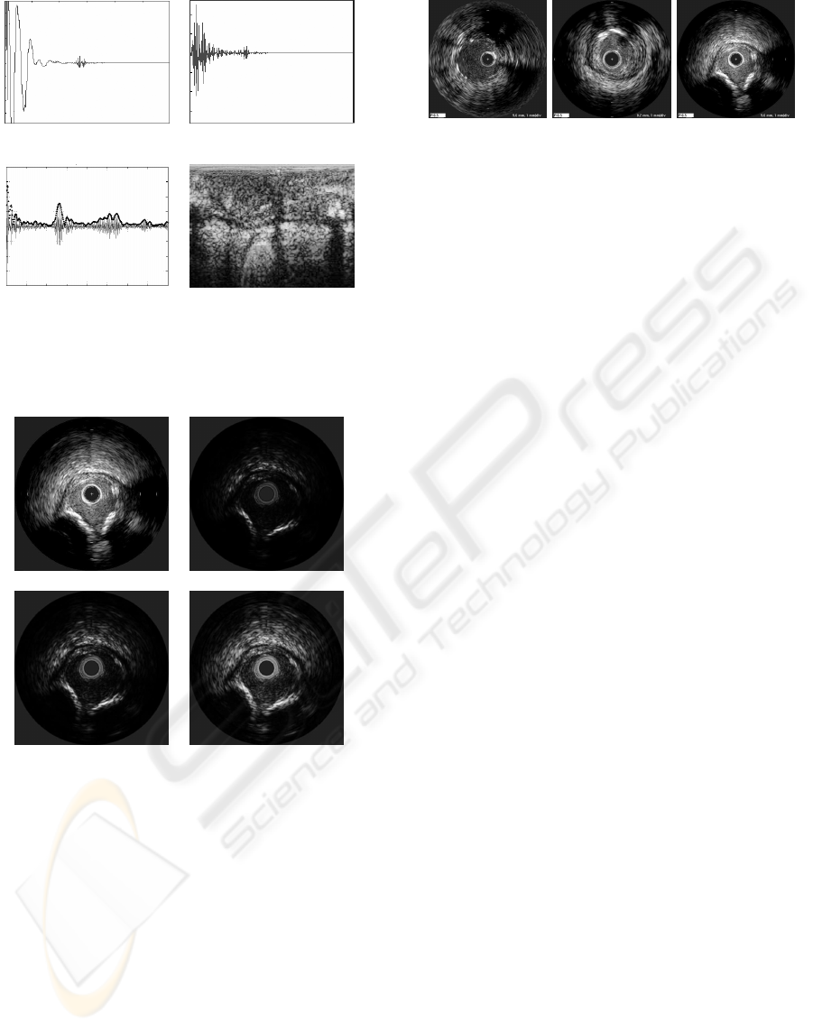
(a) (b)
(c) (d)
Figure 1: IVUS image reconstruction steps: a)RF signal ac-
quisition of an A-line, b)filtered signal c)envelope calcula-
tion from a compensated signal, d)polar image before their
cartesian construction.
(a) (b)
(c) (d)
Figure 2: IVUS images and Reconstructed IVUS im-
ages from RF signals with different DDP gain parameters.
(a)Dicom image from the IVUS equipment.(b)DDP gain
parameter fixed to 1.04. (c)DDP gain parameter fixed to
2.20. (d)DDP gain parameter fixed to 3.40.
The parameters are fixed in order to normalize im-
ages from different patients. This process allows us
to change the gain parameter of the image easily with
low computational cost. It is not an easy task in the
DICOM images since each pullback can be saved by
a different person, and the reconstruction parameters
are not usually available. Figure 2.2 shows an exam-
ple of constructed images with different gains com-
pared with a DICOM image.
(a) (b) (c)
Figure 3: Dicom images from different patients saved with
different parameter set.
3 RECONSTRUCTED IMAGE VS
DICOM IMAGE
When the IVUS study is performed, DICOM images
are generated automatically. Because of its nature,
these are recorded at one specific gain or parametriza-
tion. However, when a multiple observer study is
needed, the images can not been adjusted anymore,
since the signal information, the RF signal is lost.
To improve the visualization, DICOM images di-
minish the visibility of the outer radius in order to in-
crease the focus on the inner regions. This procedure
can hinder an automatic classification. It is because
a specific tissue can be visualized with different ap-
pearance in the inner part than in the outer part, and
from patient to patient. Figure 3 shows examples of
DICOM images from various patients recorded with
different parameter sets. Here it can be visualized an
image with the same weight over the entire depth in
(a), in (b) the contrast in the inner radius is increased,
while in (c) the outer radio is diminished. It suggests
a high variability at the time of studying various pa-
tients, since the tissue may have not the same gray
level and texture properties.
The reconstructed images represent a form of
recording all the information of the images. This
is achieved by saving the Radio Frequency Signals
coming from the IVUS equipment. In this way, im-
ages can be reconstructed using different parameteri-
zations without losing any information since any part
of the radius can be highlighted to improve the visu-
alization.
4 TEXTURE FEATURES
EXTRACTION
In order to perform a tissue characterization, features
from the image should be extracted. It has been
shown in literature that texture descriptors are robust
in presence of noise (P. Ohanian, 1992; Husoy, 1999),
as is the case of IVUS images. In this issue, we have
RECONSTRUCTING IVUS IMAGES FOR AN ACCURATE TISSUE CLASSIFICATION
115

selected three families of general texture descriptors,
Co-occurrence matrix measures, Local Binary Pat-
terns and Gabor Filter Banks. Additionally, we have
computed the presence of shading as a complemen-
tary feature.
4.1 Co-occurrence Matrix
The co-occurrence matrix can be defined as an esti-
mation of the joint probality density function of gray
level pairs in a image (P. Ohanian, 1992). The ele-
ment values in a matrix are bounded from 0 to 1 and
the sum of all element values is:
P(i, j,D,θ) = P(I(l,m) =
i⊗ I(l + Dcos(θ),m+ Dsin(θ)) = j),
where I(l,m) is the gray value at the pixel(l,m), D is
the distance among pixels and θ is the angle of each of
neighbors. The angle orientation θ has been fixed to
be [0
o
,45
o
,90
o
,135
o
], because, according to (Husoy,
1999; P. Ohanian, 1992), it is the minimum set of ori-
entations needed to describe a second-order statistic
measures of texture. After computing this matrix, six
characterizing measures, energy, entropy, the Inverse
Difference Moment, shade, inertia and Promenance
are extracted as defined in (P. Ohanian, 1992). Thus,
a 48 feature space is built for each pixel, since we are
estimating 6 different measures at 4 orientations and
two distances D = [5,8].
4.2 Local Binary Patterns
These feature extractor operators are used to detect
uniform texture patterns in circular neighborhoods
with any quantization of angular space and spatial res-
olution (Ojala and Maenpaa, 2002). They are based
on a circular symmetric neighborhood of P members
of a circle with radius R. Gray level invariance is
achieved when the central pixel g
c
is subtracted to
each neighbor g
p
, assigning to the result 1 if the dif-
ference is positive and 0 if it is negative. Each neigh-
bor is weighted with a 2
p
value. Then, the neighbors
are added, and the result is assigned to the central
pixel.
LBP
R,P
=
P
∑
p=0
s(g
p
− g
c
) · 2
p
With these operators we generate a 3 dimensional
space, by applying a radius of R = [1,2,3] and a
neighborhood of P = [8, 16,24].
4.3 Gabor Filters Bank
The Gabor Filters is an special case of wavelets
(Daugman, 1985; Feichtinger and Strohmer, 1998).
It is a Gaussian g modulated by a complex sinusoid
s. In 2D, a Gabor filter has the following form in the
spatial domain:
h(x,y) =
1
2πσ
x
′
σ
y
′
exp{−
1
2
[(
x
′
σ
x
′
)
2
+ (
y
′
σ
y
′
)
2
]} · s(x, y),
where s(x,y) and the Gaussian rotation are defined as:
s(x,y) = exp[−i2π(Ux+Vy)]
x
′
= xcosθ+ ysinθ, y
′
= −xsinθ+ ycosθ.
x
′
and y
′
represent the spatial coordinates rotated by
an angle θ. σ
x
′
and σ
y
′
are the standard deviations
for the Gaussian envelope. An aspect ratio λ and its
orientation are defined as:
λ =
σ
x
′
σ
y
′
, φ = arctanV/U
where U and V represent the 2D frequencies of the
complex sinusoid.
λ has been fixed to 1 in order to create isotropic
gaussian envelopes, that is, both σ
x
′
and σ
y
′
are equal,
and θ is discarded, θ = 0. The 2D frequency, (U,V)
have been changed to its polar representation F,φ.
Thus, we have created a filter bank using the follow-
ing parameters:
σ
x
= σ
y
= [12.7205,6.3602,3.1801, 1.5901],
φ = [0
o
,45
o
,90
o
,135
o
],
F = [0.0442,0.0884,0.1768, 0.3536],
yielding a 16 dimensional space for each pixel.
4.4 Shading
According to (Gil et al., 2006), one of the main dif-
ferences in the calcified tissue is the shadow which is
appreciated behind it. In order to detect this shadow,
we have performed an accumulative mean on a polar
image. This measure is performed by calculating the
mean, from one pixel to the end of the column. Be-
fore that, we have chosen a threshold to give the same
weight to the tissue and a smaller one to the shadows.
This differs from (Gil et al., 2006), since they want to
achieve a rough classification. This operation gener-
ates one value for each pixel.
As a result of feature extraction process, we ob-
tain a vector of 68 dimensions for each pixel, which
will be used to train the classifier. The main goal of
this is to extract the best of each technique in order to
improve the classification performance.
5 CLASSIFICATION
Once we have reconstructed and characterized the im-
age, we proceed to the classification in order to iden-
tify the different types of plaque. We have estab-
lished 3 classes of tissue: fibrotic plaque, lipid or
VISAPP 2007 - International Conference on Computer Vision Theory and Applications
116

Table 1: ECOC code map used in the classification.
Classes Classifiers
1 2 3
Calcium 1 1 0
Fibrotic Plaque -1 0 1
Soft Plaque 0 -1 -1
soft plaque, and calcified tissue. We use the Adaptive
Boosting (Adaboost) with decision stumps as super-
vised learning technique.
Adaboost allows us to add ”weak” classifiers un-
til some desired training error is obtained (Viola and
Jones, 2001; Schapire, 2001). In each step of the
algorithm a feature is chosen and assigned a certain
weight, which means how accurate this feature can
classify the training data. As a result a linear combi-
nation of weak classifiers and weights is obtained.
Since this method is generally used in order to
classify 2 classes and we have a multiclass problem,
we need to establish a criterium for the different clas-
sifiers output. This is achieved by means of Error
Correction Output Codes (ECOC) (Pujol et al., 2006).
They consist of assigning a code map table which re-
lates classifiers outputs and classes. Then, the final
classification is obtained finding the minimum dis-
tance between the resulting code and each class code-
word.
The ECOC classification map is shown in table
1. Here, the number 0 indicate that the class is not
used in the selected classifier. Because there are only
two classes left for each classifier, we apply one class
versus the other, and not one versus the rest. The
1’s indicate that the classifier should output a posi-
tive value when this class is found, and a negative one
(−1) when it is not.
Once the three classifiers results are obtained, the
Euclidean distance is found between each sample of
the test and all the class codes. Thus, the class with
the minimum codeword distance to the sample code
is assigned.
6 RESULTS
We have reconstructed IVUS images from a set of
9 patients with all the three kinds of plaque. Each
patient may have 1 or 2 vessel studies or pullbacks.
Then, for each one, 10 to 15 different vessel sections
or images are selected to be analyzed.
The experiment has been repeated nine times by
picking one patient for testing and the rest for training
at each iteration. This is done in order to avoid any
Figure 4: Classification accuracy for each type of tissue
among the different DDP gain parameters.
possible bias resulting of testing the system with the
same information as in the training set. In addition,
this gives us a roughly idea of how the classification
could behave with new unseen patients.
6.1 Tissue Segmentation
We have developed an application to construct IVUS
images from the RF signals. This has the advantage of
allowing the physicians to chose the parameters of the
reconstructed image to simplify the manual segmen-
tation task, since it permits the offline manipulation
of the images for the physicians. Although the main
purpose of this step is to segment the training data and
label it, the parameters used for the segmentation are
stored for future analysis yielding to settings normal-
ization.
The physicians have segmented from the vessel
images, 50 sections of interests per patient. These
segmentations were taken as regions of interest (ROI)
which were collected into a database categorized by
patient. These were mapped in the reconstructed im-
ages in order to construct the data set.
6.2 Classification
The performance of the classification approach was
tested by selecting 7 different DDP gain parameters
to reconstruct the images. Therefore, 7 different data
sets have been created, and their features extracted
have been processed separately. For each DDP gain
parameter value, a classification error rate has been
calculated for every type of tissue.
The accuracy for a range of DDP gain parame-
ters is shown in figure 4. Here it can be observed
that the fibrotic plaque is the most difficult to classify
compared with the other plaque types. In addition,
it is shown that the best accuracy in the 3 plaques
RECONSTRUCTING IVUS IMAGES FOR AN ACCURATE TISSUE CLASSIFICATION
117
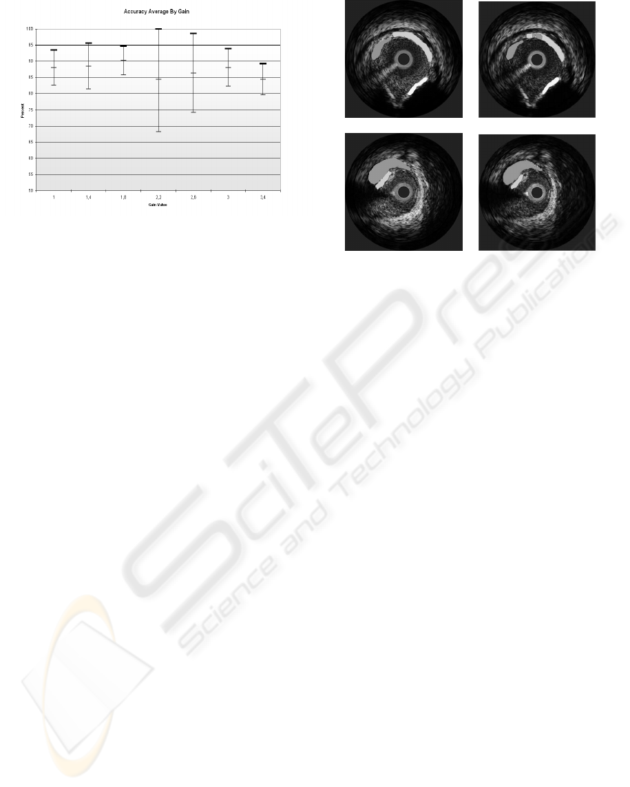
Figure 5: Global classification result among different DDP
gain parameters, with their confidence interval.
is achieved when the gain parameter is 1.8, although
there are other parameters which have better classifi-
cation accuracy for an specific plaque.
Additionally, the global accuracy and its confi-
dence interval at 90% for each gain parameter value
is calculated using all the patients. This is shown in
figure 5. In this picture we can observe that the best
classification accuracy is achieved when the gain is
equal to 1.8. This value offers us the highest average
hit rate and the smallest variability among different
patients. Note that with the gain equal to 2.2 give us
a similar accuracy rate, but the variability among the
different patients is highly significant, which can hin-
der the classification result with a unseen patient.
In any case, the accuracy rates presented here
represents an improvement in the tissue character-
ization problem with respect to the DICOM based
approaches. In this way, we can see that the re-
construction process is a critical step for classifica-
tion purposes. Usually, the classifications rates re-
ported in DICOM approaches are around of 76% of
the overall performance without any kind of postpro-
cessing(Pujol, 2004). The difference is because of the
proposed normalization procedure of the data to test
our classification framework. Figure 6 shows the re-
sult of the automatic classification using the best gain
obtained. Here it can be seen that the classification
result compared with the physician’s segmentation is
almost the same.
7 DISCUSSION AND
CONCLUSION
A method for tissue classification using IVUS recon-
structed images from raw RF data has been presented.
(a) (b)
Figure 6: Image classification result a)Image segmented by
the physician, b)Classification Result using the best gain
where white is calcified tissue, light gray fibrotic tissue and
dark gray lipid tissue.
The information used in this experiment has been ob-
tained from in vivo studies. To reduce the high vari-
ability among patients, it has been proposed a normal-
ization scheme where every image is reconstructed
with a fixed parameter set. It has been shown that DI-
COM images can not be normalized easily undermin-
ing the classification. On the other hand, by collecting
the raw RF information and reconstructing the corre-
sponding images, it is possible to establish a compar-
ative framework which reduces the inter-patient vari-
ability.
We have depicted an application of a multi-class
problem as a combination of two-class classifiers
based on discrete Adaboost using ECOC. It dimin-
ishes the ambiguity in classification when tides are
found. In addition, the use of this technique simpli-
fies this multi-class issue by reducing the amount of
data and the time of training.
It has been performed an statistical analysis to ob-
tain the best reconstruction parameters for classifica-
tion. Several values of DDP gain parameters have
been tested and their hit rate calculated to determine
which best improves the plaque classification. In ad-
dition, it has been found that the accuracy of classify-
ing reconstructed images is higher than the previously
reported using DICOM images.
The use of this framework suggests the possible
employment of different gains based on the desired
tissue. Here, it can be assigned a different parameter
set to classify each plaque, and combine them into a
global result.
VISAPP 2007 - International Conference on Computer Vision Theory and Applications
118

The classification explained has been performed
for each pixel and without any kind of postprocessing.
To generalize the response for one tissue in the image,
some grouping techniques could be applied. Addi-
tionally, by performing these, a mixed plaque com-
posed of small amounts from different tissues, can be
defined. This has not been established at class level,
since the mixed plaque is a combination of the 3 prin-
cipal plaques presented.
ACKNOWLEDGEMENTS
This work was supported in part by a research grant
from projects TIN2006-15308-C02, FIS-PI061290,
by the Generalitat of Catalunya under the FI grant and
by the Spanish Ministry of Education and Sciences
(MEC) under the FPU grant Ref: AP2005-0926
REFERENCES
Daugman, J. (1985). Uncertainty relation for resolution in
space, spatial frequency, and orientation optimized by
two-dimensional visual cortical filters. Journal of the
Optical Society of America, 2(A):1160–1169.
Feichtinger, H. G. and Strohmer, T., editors (1998). Gabor
Analysis and Algorithms: Theory and Applications.
Birkh
¨
auser.
Gil, D., Hernandez, A., Rodrguez, O., Mauri, F., and
Radeva, P. (2006). Statistical strategy for anisotropic
adventitia modelling in ivus. IEEE Trans. Medical
Imaging, 27:1022–1030.
Gonzales, R. and Woods, R. (1992). Image Processing.
Adison - Wesley.
Husoy, T. R. J. H. (1999). Filtering for texture classification:
A comparative study. IEEE Transactions on Pattern
Analysis and Machine Intelligence, 4:291–310.
Ojala, T. and Maenpaa, M. P. T. (2002). Multiresolution
gray-scale and rotation invariant texture classification
with local binary patterns. IEEE Transactions on Pat-
tern Analysis and Machine Intelligence, 24:971–987.
P. Ohanian, R. D. (1992). Performance evaluation for
four classes of textural features. Pattern Recognition,
25:819–833.
Pujol, O. (2004). A semi-supervised Statistical Framework
and Generative Snakes for IVUS Analysis. Graficas
Rey.
Pujol, O., Radeva, P., and Vitria, J. (2006). Discriminant
ecoc: A heuristic method for application dependent
design of error correcting output codes. IEEE Trans-
actions on Pattern Analysis and Machine Intelligence,
28:1001–1007.
Schapire, R. (2001). The boosting approach to machine
learning: An overview.
Viola, P. and Jones, M. (2001). Robust real-time object de-
tection. In CVPR01, volume 1, page 511.
RECONSTRUCTING IVUS IMAGES FOR AN ACCURATE TISSUE CLASSIFICATION
119
