THEORETICAL FOUNDATIONS OF 3D SCALAR FIELD
VISUALIZATION
Mohammed Mostefa Mesmoudi
Department of Mathematics, University of Mostaganem, Po. Box 227, Route BelHacel, Mostaganem 27000, Algeria
Leila De Floriani
Department of Computer Science, University of Genova, Via Dodecaneso n 35, 16146 Genova, Italy
Paolo Rosso
Department of Information Systems and Computation, Polytechnic University of Valencia
Camino de Vera s/n, 46022 Valencia, Spain
Keywords:
3D Visualization, geometric modeling, morphology extraction, image segmentation, watershed transform,
multiresolution.
Abstract:
In this paper we introduce two novel technics that allow for a three dimensional scalar field to be visualized
in the three dimensional space R
3
. Many applications are possible especially in medicine imagery. New
multiresolution models can be build based our techniques. Moreover, we show that these two visualization
techniques allow the extraction of morphological features of the space and that may not be captured by classical
methods.
1 INTRODUCTION
In many applications of computer graphics (e.g.,
medicine imaging) the visualization of scalar fields
is a basic tool to explore and understand the structure
of the field. Visualization of 3D scalar fields needs
an additional dimension to be achieved. This is im-
possible to do in R
3
from the Cartesian point of view
since our visual perception is limited to three parame-
ters. To overcome this problem, we need to tackle the
problem from a different point of view.
Smooth Morse theory is the basic tool used to extract
morphological features of a domain endowed with a
scalar field (Smale, 1960). The domain is decom-
posed into stable and unstable components. Stable
components are associated with minima, while un-
stable components are associated with maxima. In
the discrete case algorithms have been proposed to
extract morphological features with similar proper-
ties as in Morse theory. A large part of such tech-
niques deal with 2D scalar fields case, see, for in-
stance, (Bajaj et al., 1998), (Bajaj and Shikore, 1998),
(Edelsbrunner et al., 2001), (J.Toriwaki and Fuku-
mura, 1975), (Nackman, 1984), (Peucker and Dou-
glas, 1975), (Watson et al., 1985). The watershed
transform introduced by Vincent et al. in (Vincent
and Soille, ), for 2D scalar fields considers the graph-
ical representation of a 2D scalar field as a surface
that will be immersed progressively in water. Catch-
ment basins, which correspond to stable Smale de-
composition in Morse theory, are constructed and sur-
face segmentation is, hence, performed. Very few pa-
pers deal with 3D (and 4D) scalar fields. This is due
to difficulty of applying, in the discrete, Morse the-
ory to 3D (and 4D)scalar fields. In (H. Edelsbrunner,
2003), an algorithm for the construction of Smale-
decomposition for linear piece-wise linear functions
on a three dimensional domain is presented. Man-
gan et al., gave in (Mangan and Whitaker, 1999) a
watershed algorithm that segments a 3D surface into
patches. Their algorithm is based on the total curva-
ture of the surface approximated at the vertices of the
mesh approximating the surface.
Here, we present two coupled novel techniques
that allow visualizing 3D scalar fields in the Euclid-
ean three-dimensional space. These novel techniques,
that we call AUBL and PGR, are based on some
fundamental geometric properties of surfaces and
69
Mostefa Mesmoudi M., De Floriani L. and Rosso P. (2007).
THEORETICAL FOUNDATIONS OF 3D SCALAR FIELD VISUALIZATION.
In Proceedings of the Second International Conference on Computer Vision Theor y and Applications, pages 69-77
DOI: 10.5220/0002065300690077
Copyright
c
 SciTePress

on their embedding the Euclidean three-dimensional
space. AUBL and PGR visualization techniques have
the advantage of representing a 3D scalar field in a
natural and intuitive way and allow extracting mor-
phology features of the field that may not be captured
by classical methods. Hence, we obtain a natural gen-
eralization, to 3D scalar fields, of the watershed trans-
form. In addition, AUBL and PGR techniques pro-
vide a new approach to study a 3D scalar field us-
ing additional tools like curvature of the surface or of
the field, and dependencies under elementary trans-
formation (e.g., time evolution of a pathology) and
that were not possible with classical methods. AUBL
and PGR can be used as a support for data mining
visualization of 4D scalar fields. Study of 4D scalar
fields goes beyond the scope of this paper whose aim
is to present the mathematical foundations of AUBL
and PGR techniques. Many applications of AUBL and
PGR are possible in 3D visualization, especially in
medical imaging New multi-resolution models based
on AUBL technique can be build. We will discuss this
possibility in the paper. Roughly speaking, the AUBL
technique represents the scalar field as an atmosphere
over the domain and PGR represents the depth of the
upper layer of the atmosphere.
The remainder of this paper is organized as follows.
In the next Section we present some background no-
tions related to the basic mathematical notions needed
in this paper. In Section 3, we present the fundamental
geometric property from which we derive the AUBL
and PGR visualization algorithms. We will discuss
how algorithms AUBL and PGR can be used to ex-
tract and visualize morphological features of a field
that may not be detected through other classical tech-
niques. In Section 4, we describe how AUBL visual-
ization technique can generalize the watershed trans-
form to extract the morphological feature. In the last
Section, we draw some concluding remarks and we
discuss our ongoing work.
2 BACKGROUND
In this Section, we present the basic mathematical no-
tions that we need to develop the paper material.
2.1 Geometry and Topology of
2-Manifolds
Two dimensional manifolds (without boundary) are
surfaces that are locally diffeomorphic to discs of R
2
.
Around any point p of a surface S, one can find a
neighborhood U of p and a diffeormorphism φ that
maps a disc in R
2
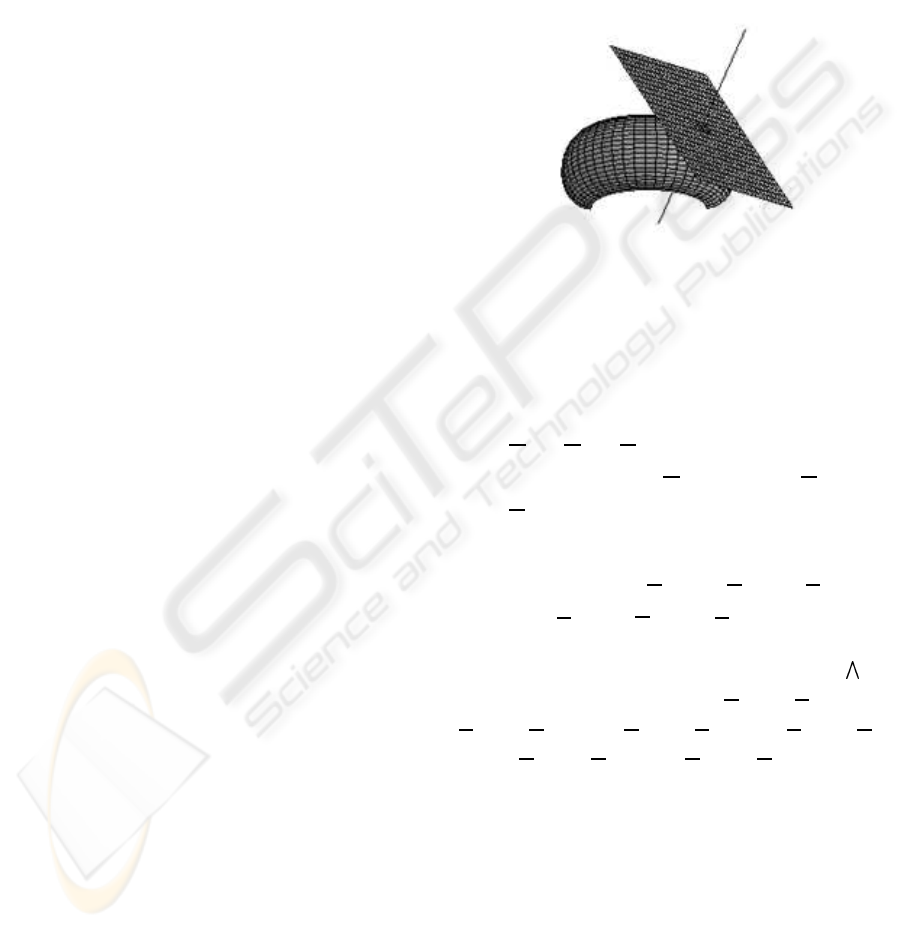
on U. At each point p of a surface S,
a tangent plane T
p
S is defined and thus a normal vec-
tor
−→
N
p
to S at point p can be drawn. Vector
−→
N
p
gener-
ates a 1-dimensional vectorial space <
−→
N
p
>. Hence,
the Euclidean 3-dimensional space R
3
is retrieved in
the direct sum T
p
S⊕ <
−→
N
p
> of vectorial spaces T
p
S
and <
−→
N
p
>, see Figure 1.
If the surface S is described by an equation
Figure 1: A surface with its tangent plane and normal vec-
torial space at a point.
f(x, y,z) = 0 (e.g., x
2
+ y
2
+ z
2
− 1 = 0 for the unit
sphere), then coordinates of the normal vector
−→
N
p
to S at a point p are given by the partial deriva-
tives (
∂f
∂x
(p),
∂f
∂y
(p),
∂f
∂z
(p)). The tangent plane is de-
scribed by the equation
∂f
∂x
(p)(x − x
p
) +
∂f
∂y
(p)(y −
y
p
) +
∂f
∂z
(p)(z − z
p
) = 0. If surface S is described
by a parametric relations S = {(x(t,s),y(t,s),z(t, s)) :
(t, s) ∈ D ⊂ R
2
}, then tangent plane is generated by
the two vectors
−→
V
p
= (
∂x
∂t
(t
0
,s
0
),
∂y
∂t
(t
0
,s
0
),
∂z
∂t
(t
0
,s
0
))
and
−→
V
′
p
= (
∂x
∂s
(t
0
,s
0
),
∂y
∂s
(t
0
,s
0
),
∂z
∂s
(t
0
,s
0
)) with p =
(x(t
0
,s
0
),y(t
0
,s
0
),z(t
0
,s
0
)). Then the normal vec-
tor
−→
N
p
is equal to the vectorial product
−→
V
p
−→
V
′
p
whose coordinates are given by (
∂y
∂t
(t
0
,s
0
)
∂z
∂s
(t
0
,s
0
) −
∂z
∂t
(t
0
,s
0
)
∂y
∂s
(t
0
,s
0
);−
∂x
∂t
(t
0
,s
0
)
∂z
∂s
(t
0
,s
0
) +
∂z
∂t
(t
0
,s
0
)
∂x
∂s
(t
0
,s
0
);
∂x
∂t
(t
0
,s
0
)
∂y
∂s
(t
0
,s
0
) −
∂y
∂t
(t
0
,s
0
)
∂x
∂s
(t
0
,s
0
)). For
more details, we refer to any book of differential
geometry (e.g., (Berger and Gostiaux, 1972), (Spivak,
1979) ).
Two surfaces are said be topologically equivalent if
they are homeomorphic. Algebraic topology classi-
fies compact surfaces by their genus and orientabil-
ity, see (Massey, 1977). The genus g is the number
of handles in a surface. A topological sphere S
2
has
null genus since it has no handle, while a torus T
2
has
genus 1, since it has exactly one handle. To obtain
surfaces of a higher genus g ≥ 2, we consider the con-
nected sum of g tori (T
2
#T
2
#.. .#T
2
). The connected
VISAPP 2007 - International Conference on Computer Vision Theory and Applications
70

sum is defined by the quotient space of an equivalence
relation that identifies (i.e., glue) the boundary points
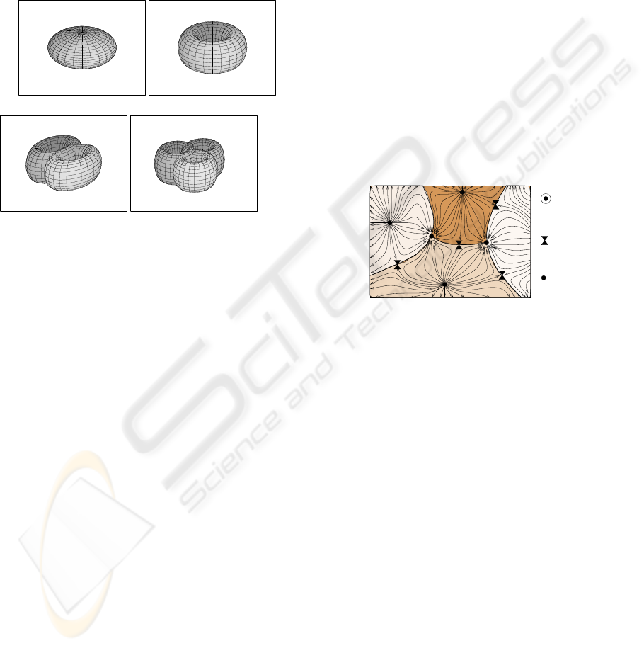
of two holes created on two consecutive tori. In Fig-
ure 2, we give an illustration of such surfaces with
genus 0, 1, 2 or 3. A compact surface with non empty
boundary components can be obtained from the previ-
ous described surfaces by cutting along closed curves.
In the remainder of this paper we consider only ori-
entable surfaces.
(a) (b)
etc...
(c) (d)
Figure 2: Surfaces of genus 0 in (a), 1 in (b), 2 in (c) and 3
in (d), and so on.
2.2 Morse Theory
A Morse function on a manifold M is a C
2
-
differentiable real-valued function f defined on M
such that its critical points are non-degenerate (Mil-
nor, 1963). This means that the Hessian matrix Hes
P
f
of the second derivatives of f at any point P ∈ R
d
on
which the gradient of f vanishes(Grad
P
f = 0) is non-
degenerate (Det(Hes
P
f 6= 0). Morse (Milnor, 1963)
has proven that there exists a local coordinate system
(y
1
,...,y
n
) in a neighborhood U of any critical point
P, with y
j
(P) = 0, for all j = 1, ... ,n, such that the
identity
f = f (P) − (y
1
)
2
− ... − (y
ı
)
2
+ (y
ı+1
)
2
+ ... + (y
n
)
2
holds on U, where ı is the number of negative eigen-
values of Hes
P
f, and it is called the index of f at P.
The above formula implies that the critical points of a
Morse function are isolated. This allows us to study
the behaviour of f around them, and to classify their
nature according to the signs of the eigenvalues of the
Hessian matrix of f. If the eigenvalues are all pos-
itives, then the point P is a strict local minimum (a
pit). If the eigenvalues are all negatives, then P is a
strict local maximum (a peak). If the index ı of f at
point P is different from 0 and n, then the point P is
neither a minimum nor a maximum, and, thus, it is
called an ı-saddle point (a pass).
The decomposition of the manifold domain as-
sociated with f, introduced by Thom (Thom, 1949)
and followed by Smale (Smale, 1960) is based on the
study of the growth of f along its integral curves. An
integral curve is a curve which is every where tan-
gent to the gradient vector field. Integral curves orig-
inating from a critical point of index ı form a ı-cell
C
s
, called a stable manifold. In the same way inte-
gral curves converging to a critical point of index ı
form a dual (n− ı)-cell C
u
, called an unstable man-
ifold. Stable manifolds are pairwise disjoint and de-
compose the field domain M into open cells, (see Fig-
ure 3). The cells form a complex, as the boundary
of every stable manifold is the union of lower dimen-
sional cells. Similarly, the unstable manifolds decom-
pose M into a complex dual to the complex of sta-
ble manifolds. Integral curves connecting saddles to
other critical points are called separatrices.
Maximum
Minimum
Saddle
Figure 3: Decomposition of a domain into four stable 2-
manifolds.
3 3D SCALAR FIELDS
VISUALIZATION
By 3D scalar field we mean a scalar field defined on
any smooth surface embedded in R
3
. Such surfaces
may have non-null genus, may contain boundary
components, may be compact, open, etc...
The basic idea underlying our new technique is to use
a fundamental geometric property of the representa-
tion of 2D scalar fields in the 3D Euclidean space. Let
us discuss first the graphical representation of a scalar
field f defined on a domain D of R
2
. The graphi-
cal representation of f over D is a surface S defined as
S = {(x,y,z) : (x,y) ∈ D and z = f(x, y)} (1)
The domain D in R
3
is embedded onto a set
˜
D =
{(x,y, 0) : (x,y) ∈ D} and a point p(x,y) in D is sent
THEORETICAL FOUNDATIONS OF 3D SCALAR FIELD VISUALIZATION
71

to point ˜p(x,y, 0) in
˜
D. Also, domain
˜
D has a para-
meterization through points of D. Hence, function f
can be seen as a 3D scalar field
˜
f defined on
˜
D by :
˜
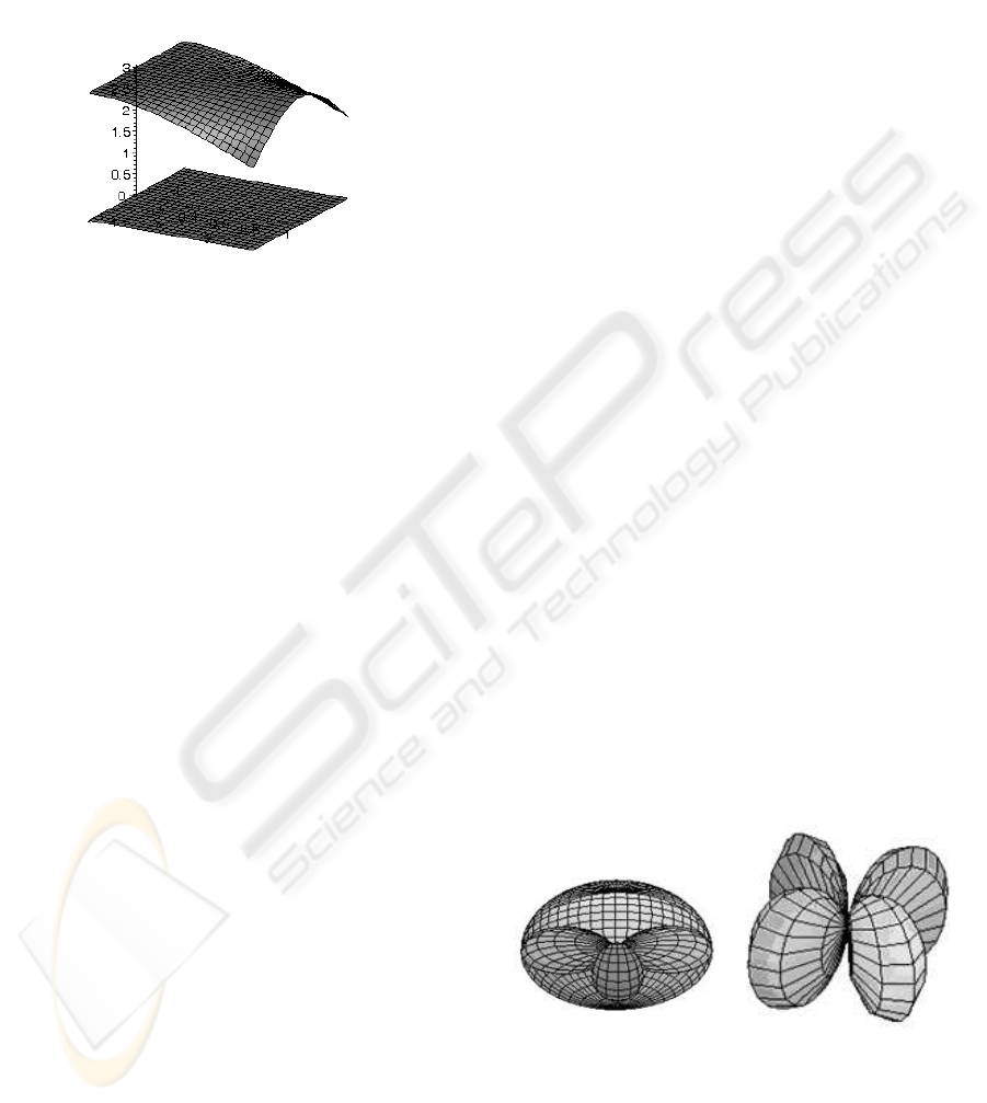
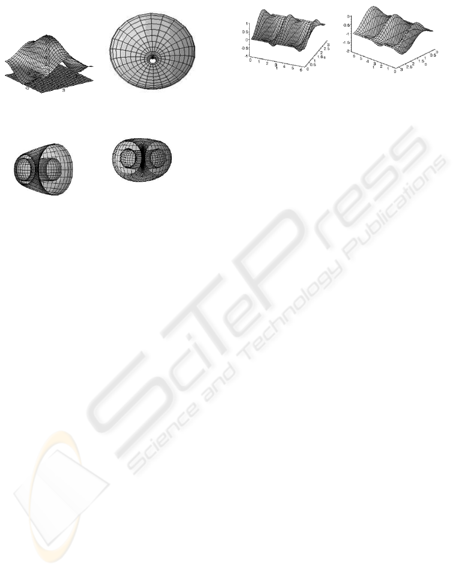
f( ˜p) = f(p). In Figure 4, we illustrate such situation.
Figure 4: Graphic representation of f(x,y) =
˜
f(x,y,0) =
cos(xy) over the Domain D = [−π/2,π/2] × [0,π/3] ≃
[−π/2,π/2] × [0,π/3] × {0} =
˜
D.
Property 1 (The first key Property.) For a given
point ˜p in
˜
D, vector
−−−→
˜p
˜
f( ˜p) is normal to
˜
D and k
−−−→
˜p
˜
f( ˜p) k=| f( ˜p) |.
This is due to the fact that the canonical basis of R
3
is
orthonormal and (0,0, f(x,y)) are the coordinates of
vector
−−−→
˜p
˜
f( ˜p).
Generalizing the idea in property 1, we can give a
first graphical representation of 3D scalar fields. Let
S be an embedded smooth surface in R
3
and f be a
scalar field defined on S. The graphical represen-
tation of function f would be a subset of R
4
defined by
G = {(x,y,z,t) : (x,y, z) ∈ S and t = f(x,y,z)} (2)
Since we cannot visualize items in R
4
, Property 1
allow us to visualize both S and its image by f in R
3
as in Figure 4.
First Visualization principle.
Definition 1 Let
−→
N
p
be the unit normal vector of S at
point p. The graphical representation of scalar field
f over S is the surface S ⊂ R
3
defined by:
S = {p+ f(p)
−→
N
p
: p ∈ S} (3)
To represent the image of point p ∈ S, the pre-
vious definition associates p with the point
˜
f(p) := p + f(p)
−→
N
p
. Then, vector
−−−→
p
˜
f(p) is normal
to S at p and k
−−−→
p
˜
f(p) k=| f(p) | Thus, Property 1
is satisfied. The graphical representation of function
f defines an atmosphere layer over surface S. The
thickness of the layer is given by the function values.
As an example, the graphical representation of a
constant function over a sphere is a larger sphere with
the same center and in which the radius is augmented
by the constant value of the function.
Definition 2 When surface S is included in the inte-
rior space bounded by S we say that S has a positive
f-atmosphere. When the reverse holds, we say that S
has a negative f -atmosphere.
When the new surface S is topologically equivalent to
S, we can always inflate or deflate surface S (without
losing the perpendicularity property) so that S ∩S =
/
0
and obtain positive, or negative atmosphere follow-
ing the need of the user to get a best representation
scheme. Inflation (resp: deflation) can be performed
by translating
˜
f(p) in the direction of the normal vec-
tor
−→
N
p
by a constant positive (resp. negative) value.
Formal definitions of inflation and deflation are given
in section 4. To avoid self-intersections of S due to
limitation of available space in the interior of even-
tual handles of the surface S, we can change the scale
of the normal vector
−→
N
p
by a multiplicative smaller
constant value.
When the topology equivalence between S and S is
not satisfied, we can only deflate S to include it in
the interior space of S and, hence, obtain a nega-
tive atmosphere. In Figure 6, we illustrate the above
situation for the unit sphere x
2
+ y
2
+ z
2
= 1 with
a negative atmosphere corresponding to the function
f(x, y,z) = x
2
− y
2
− 1.
(a) (b)
Figure 5: In (a), a plane section representing the unit sphere
with a negative atmosphere defined by a function f(x,y,z) =
x
2
− y
2
− 1. In (b), the visualization of S corresponding to
˜
f.
VISAPP 2007 - International Conference on Computer Vision Theory and Applications
72

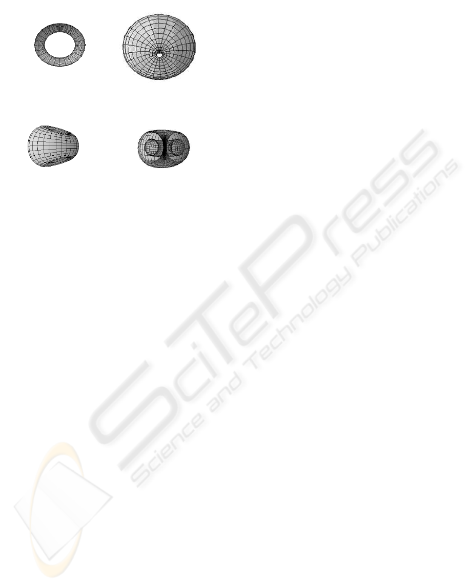
(a) (b)
(c) (d)
Figure 6: In (b)and (c): The graphical representation of Ox-
height function f(x, y,z) = x of a torus T
2
(in (a)) whose
revolution axis is Oz. In (d), we represent a section of
the height function representation: The torus and its f -
atmosphere are Shown.
Definition 3 Under such assumptions, we call the
graphical representation S of f, the atmosphere up-
per bound layer (AUBL) of the pair (S, f).
In Figure 6, we illustrate the atmosphere of Ox-height
function defined on a torus T
2
whose revolution axis
is Oz (i.e., f(x, y,z) = x for all points (x,y, z) ∈ T
2
).
Second Visualization Principle.
AUBL visualization can be completed by a second
visualization technique based on a graph represen-
tation of f over flat subset D ∈ R
2
. This can be
realized by composing f with a (local) coordinates
system on S. Of course, this second visualization
does not represent directly f over S, but it has some
advantages:
• This representation provides additional informa-
tion on the morphology of the surface that can
be easily captured by the different existing tech-
niques since it is based on 2D scalar field visual-
ization.
• The AUBL visualization technique described
above depends on the geometry of surface S.
Hence, a negatively (resp. positively) curved
hump on S may produce a negatively (resp. pos-
itively) curved hump on S . Then function f may
have a decreasing (resp. increasing) appearance,
while, in reality, f has the opposite growth. To
compensate this issue, we consider the growth of
f over a flat domain of R
2
. Composing f with φ
and then representing the resulting function over
D solves this issue.
From an other point of view, the above discussed
humps that appear on S represent interesting re-
gions related to the morphology of the surface
and that may correspond to some kind of critical
points of the vector function
˜
f and/or f. Thus,
additional morphology information is captured by
AUBL visualization that cannot be seen by stan-
dard tools.
Let {φ(t,s) = (x(t,s),y(t,s),z(t, s)) : (t, s) ∈ D} a
local (or a global) parameterization of S over a do-
main D ∈ R
2
.
Definition 4 We call the visualization of f ◦ φ over D
by the parametric growth representation (PGR) of f
over S.
Hence, a complete understanding of f will be
achieved by coupling together both visualizations
AUBL and PGR.
In Figure 7, we provide an illustration of (AUBL,
PGR)-visualizations of the (Ox)-height scalar field
defined on torus T
2
parameterized by (t,s) where t is
the angle between axis (Ox) and
−→
Op
′
where p
′
is the
projection a current point p on T
2
. Parameter s is the
angle between axis (Oz) and
−→
Op. The PGR represen-
tation shows that setting parameter s = s
0
, function
f ◦ φ(t,s
0
)) increases, reaches a maximum and then
decreases. Similar behaviour happens by fixing first
t.
In the following example, we consider the case of
a function which is not Morse with two degenerated
points. We will show how PGR visualization tech-
nique can be applied to extract 6 critical points on a
surface. In Section 4, we will show how AUBL visu-
alization technique can be applied to retrieve the same
critical points with the critical net in addition.
Example. Let us consider function f(x,y, z) = x
2
−y
2
defined on the unit sphere S
2
. Gradient vector field
at any point p = (x,y,z) ∈ R
3
is given by Grad
p
f =
(2x,−2y,0). The gradient field vanishes on the set
{(0,0,z) :∈ R}. The Hessian matrix Hes
p
f of f
at point p is generated by column vectors (2,0,0),
(0,−2,0) and (0, 0,0). Matrix Hes
p
f is clearly de-
generate at any point p ∈ R
3
. Hence f is not a Morse
function. Thus, we can not apply techniques of Morse
theory to study f.
Let us parameterize the unit sphere with it spher-
ical coordinates x = cos(t)sin(s), y = sin(t)sin(s)
and z = cos(s), where t ∈ [0,2π] is the angle in
(Oxy)-plane attached to the (Ox)-axis. Parameter
s ∈ [0,π] is the angle attached to (Oz)-axis. A simple
computation gives
˜
f(t,s) = f(x(t,s),y(t,s),z(t, s)) =
THEORETICAL FOUNDATIONS OF 3D SCALAR FIELD VISUALIZATION
73

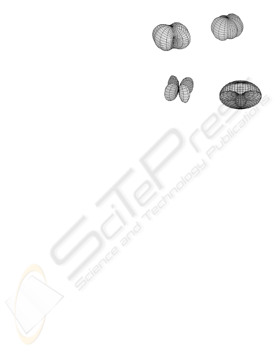
(a) (b)
(c) (d)
Figure 7: In (a) the PGR and, in (b), the AUBL
visualizations of Ox-height function f(x,y,z) = x
of torus T
2
= {(x(t,s), y(t,s), z(t,s)) : x(t,s) =
(2 + cos(s))cos(t);y(t,s) = (2 + cos(s))sin(t);z(t,s) =
sin(s) : (t, s) ∈ [−π,π]
2
}. In (c), an atmosphere section
at t = 0 and at t = π. In (d), an atmosphere section at
t = −π/2 and at π/2 .
cos(2t)sin
2
(s). The gradient vector field of
˜
f at a
point u = (t,s) is given by
Grad
u
˜
f = (−2sin(2t)sin
2
(s),cos(2t)sin(2s)).
The gradient of
˜
f vanishes on the set
Crit
˜
f = {(t,0),(t,π) : t ∈ [0,2π]} ∪
{(0,0),(π/2,π/2),(π,π/2),(3π/2, π/2}. On the
unit sphere, points in the first set of Crit
˜
f of type
(t, 0) correspond to the north pole (0,0,1), and to the
south pole (0,0,−1) for points of type (t,π). Points
in the second set of Crit
˜
f corresponds respectively to
(1,0,0), (0,1,0), (−1,0, 0) and (0,−1,0).
The Hessian matrix of
˜
f is generated by vec-
tors (−4cos(2t)sin
2
(s),−2sin(2t)sin(2s)) and
(−2sin(2t)sin(2s),2cos(2t)cos(2s)). Simple com-
putation implies that Hes
u
˜
f is degenerate for
points of type (t,0) and (t,π) that corresponds
to north and south poles of the sphere. For the
other four points, the Hessian Hes
u
˜
f is non de-
generate and has determinant equal to 8 (≥ 0)
at each point. This implies that each point in
{(0,0),(π/2,π/2),(π,π/2),(3π/2, π/2} is either a
maximum or a minimum. Thus maxima and minima
of f on the unit sphere correspond to (1,0,0),
(0,1,0), (−1,0,0) and (0, −1,0). A simple compu-
tation gives a maximal value 1 of f at points (1,0,0)
and (−1, 0,0) and a minimal value −1 of f at points
(a) (b)
Figure 8: In (a), PGR visualization of the function
f(x,y,z) = x
2
− y
2
over the unit sphere. Maxima and min-
ima appear alternatively. There are two minima and one
maximum in the interior of the surface. Two maxima appear
on the boundary segments t = 0, t = 2π but they correspond
to the same point on the unit sphere. Function f ◦ φ, has a
constant value on segments s = 0, s = π. Points on these
boundary segments are critical, they correspond all to the
north or the south pole. In (b), the PGR visualization of the
function f(x,y,z) = x
2
− y
2
− 1. The shapes of surfaces in
(a) and in (b) are identical. This is not the case with AUBL
visualization technique, see Figure 9(a) and (c).
(0,1,0) and (0,−1,0). Hence, north and south poles
of the sphere are degenerate saddles and f vanishes
on them ( f(0, 0,1) = f(0,0, −1) = 0). The PGR
visualization of function f is illustrated in Figure
8(a).
4 MORPHOLOGY EXTRACTION
BASED ON AUBL
INFLATION/DEFLATION
The distance between a point p and its image (on
AUBL, PGR or in the standard cartesian case) is given
by | f(p) |. Points for which this distance is mini-
mal correspond to minima and points for which this
distance is maximal correspond to maxima. In this
section we will give a method that extracts those crit-
ical points with saddle and the critical net on surface
S associated with function f. To begin, let us give a
formal definition of inflation and deflation.
Definition 5 Suppose that normal vectors
−→
N
p
are di-
rected towards the exterior of S. Inflation process is a
dynamical system Inflat : S ×[0, +∞[→ R
3
that asso-
ciates a pair (
˜
f(p),t) with In flat(
˜
f(p),t) =
˜
f(p) +
t
−→
N
p
.
Deflation process is a dynamical system De flat :
S ×]−∞,0] → R
3
that associates a pair (
˜
f(p),t) with
Deflat(
˜
f(p),t) =
˜
f(p) − t
−→
N
p
.
For each instant t
0
, In f lat(S ,t
0
) (resp. Deflat(S ,t
0
))
is a surface S
t
0
obtained from S by translating all
points
˜
f(p) along vectors
−→
N
p
by constant value
VISAPP 2007 - International Conference on Computer Vision Theory and Applications
74

t
0
. In Section 3, we have seen that inflation and
deflation of the atmosphere permit to get positive
and negative atmospheres over the surface S. This
inflation/deflation process has an important property
in capturing the morphology of surface S. This is
given by
Property 2 (The second key Property). While per-
forming an inflation/deflation, imprints of crossing
surface S at a given time t
0
defines level sets S ∩ S
of f over S at moment t
0
.
Proof. At instant t
0
, intersection of surface S
t
0
with S
is given by the set of points {p ∈ S :
˜
f(p)∓t
0
−→
N
p
= p}.
Substituting
˜
f(p) by its value, we have S
t
0
∩S = {p ∈
S : p + f(p)
−→
N
p
∓ t
0
−→
N
p
= p} which gives S
t
0
∩ S =
{p ∈ S : f(p) = ±t
0
}. This is equivalent to say
S
t
0
∩ S = f
−1
(±t
0
). Thus level sets at instant t
0
are
simply S
t
0
∩ S.
This property generalizes the watershed transform for
2D scalar fields. The watershed transform extracts
morphology features of 2D scalar fields by crossing S
parallel planes z = constants. In the 3D scalar field
case, minima and maxima of f are obtained when
S and S
t
0
intersect tangentially. In case of non de-
generate points, we obtain, at moment t
0
, isolated
points. And in case, of degenerate points we obtain
sub-surface patches. After the detection moment of
local minima (or maxima), circles are created and cor-
respond to level sets of the function. When the infla-
tion/deflation process continue in time, circles grow
up on S until a moment in which an intersection be-
tween circles holds. At this moment, saddle points are
obtained. When pursuing inflation/deflation process
small time after, obtained saddle points split out and
the previous circles merge together. Level circles
propagate with time on S and the splitted points fol-
low integral lines an describe the critical net of f over
S (i.e., integral lines that are separatrices). Hence, the
morphology of S is captured naturally by the infla-
tion/deflation process.
In Figures 9 and 10, we represent the infla-
tion/deflation process, at different moments, of func-
tion f(x,y,z) = x
2
− y
2
defined over the unit sphere
S
2
. Critical points of f and the critical net on S
2
ap-
pear naturally by the inflation/deflation process here.
Critical net is formed by two orthogonal big circles
on S
2
obtained from the intersection between S
2
with
planes x = 0 and y = 0), see Figure 10(m).
We have seen in Section 3 that this function is not
Morse and the study of PGR visualization implies
four non degenerate points (2 maxima and 2 minima),
and two degenerate points at north and south poles of
the sphere. These poles are two (degenerate) saddle
(a) (b)
(c) (d)
Figure 9: Inflation/Deflation process of function f(x,y,z) =
x
2
− y
2
defined over the unit sphere S
2
: In (a), surface S
alone is depicted while in (b) AUBL visualization of S and
S is shown. In(c), the completely deflated S is represented.
In (d), a section showing the completely deflated scheme
inside the unit sphere. The two intersection points of the
unit sphere with the deflated surface are critical points of
the same nature (minima or maxima).
points. We retrieve here this result plus the critical
net. Four Regions (stable and unstable components)
representing Morse complex on the unit sphere are,
thus, obtained.
Remarks.
• Under the inflation/deflation process, the scalar
field is simply translated. Thus, the shape of
the surface obtained from the PGR visualization
of the field is the same. The surfaces is simply
translated positively (inflation) or negatively (de-
flation), see Figure 8.
• In AUBL visualization, the shape of surface S
depends continuously on the inflation/def-lation
process, see Figure 10. This is due to the fact
that the original surface S is curved. From an-
other point of view, this is a remarkable fact, since
it will give more flexibility to the user to work
with the field under translations or homotheties.
This will open other perspectives to study the
fields with other approaches (constraint on field
(i.e.,S ) curvature, ...). In medicine applications,
the shape evolution, with time, of a pathological
organ can be predicted with the inflation/deflation
process (i.e, by translating the field by constants
(time)). And hence consequences can be pre-
dicted, see Figure 11.
THEORETICAL FOUNDATIONS OF 3D SCALAR FIELD VISUALIZATION
75

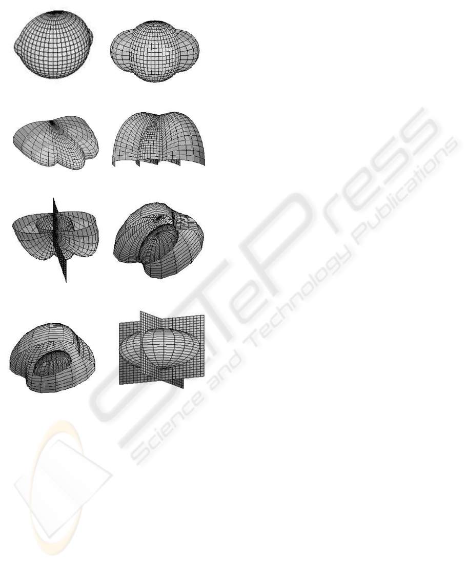
(e) (g)
(h) (i)
(j) (k)
(l) (m)
Figure 10: In(e), the beginning of the inflation process of
S . Unit sphere intersects the inflated surface at two created
circles representing levels sets of f . In (g), the growing
process of level sets (circles) appear clearly. In (h), the max-
imal growing of the two circles. Their intersection points
are a saddles (north and south poles). In (i), each saddle
point is splitted into 2 points to allow the previous circles
to merge together in one curve that appear clearly. In (j),
the splitted points follow the plane x = 0 and describe a big
circle on the unit sphere. In (k), the ultimate intersection be-
tween S
2
and the inflated surface. In (l), pursuing inflation,
we obtain a positive atmosphere around the unit sphere. In
(m), the critical net corresponds to big circles obtained by
the intersection of S
2
with planes x = 0, y = 0. Plane y = 0
corresponds to section in (d). Four Regions representing
stable and unstable Smale-decomposition components are,
thus, obtained.
• The curvature of the field (i.e., of surface S) tends
to 0 with inflation ( positive translations). The
classical methods do not approach fields from
this point of view, since translations and homo-
theties do not have a significant importance from
the Cartesian point of view. From our point of
view this fact gives a coarse vision of the original
field, see Figure 11. An application of AUBL to
multi-resolution is conceivable from this point of
view. Each resolution level corresponds to a trans-
lation value c. Coarse levels are obtained when
c increases (inflation), and refined level appear
when c decreases towards zero (deflation). The
original surface is obtained for c = 0. Moreover,
this multi-resolution process can be applied to the
original surface S with function f = 0 (in this case
we have S = S ) to produce multi-resolution mod-
els of surface S. We can also apply it to any func-
tion f to get multi-resolution models of surface
S . We can find a correspondence between infla-
tion and the reduction process of the mesh, since
the simplification process reduces the number of
triangles and curvature tends to zero on larger re-
gions. We can also find correspondence between
deflation and refinement process, since this later
increases the number of triangles and the curva-
ture takes more precise values.
5 CONCLUDING REMARKS
We have presented two novel techniques AUBL and
PGR that allow visualization of 3D-scalar fields in the
Euclidean space R
3
. AUBL and PGR techniques are
coupled together to give a complete comprehensive
representation of 3D scalar fields. We have pointed
out other advantages of (AUBL,PGR) that allow the
extraction of additional morphological features of the
domain that may not be captured by classical tools. A
method, based on AUBL, generalizing the watershed
transform has been presented and detailed with an ex-
ample. In our ongoing work, we will adapt AUBL
technique for meshes and we will develop a visual-
izing tool that allow the user to interact with both
AUBL and PGR techniques at the same time. More-
over, we will develop algorithms for the generalized
watershed transform to extract morphology features
of 3D scalar fields. We plan also to investigate the
possibility of applying our approach in the visual data
mining field. The idea is to enhance the segmental
visualization technique (Ankerst, 2000) over a sphere
divided into sectors.
VISAPP 2007 - International Conference on Computer Vision Theory and Applications
76

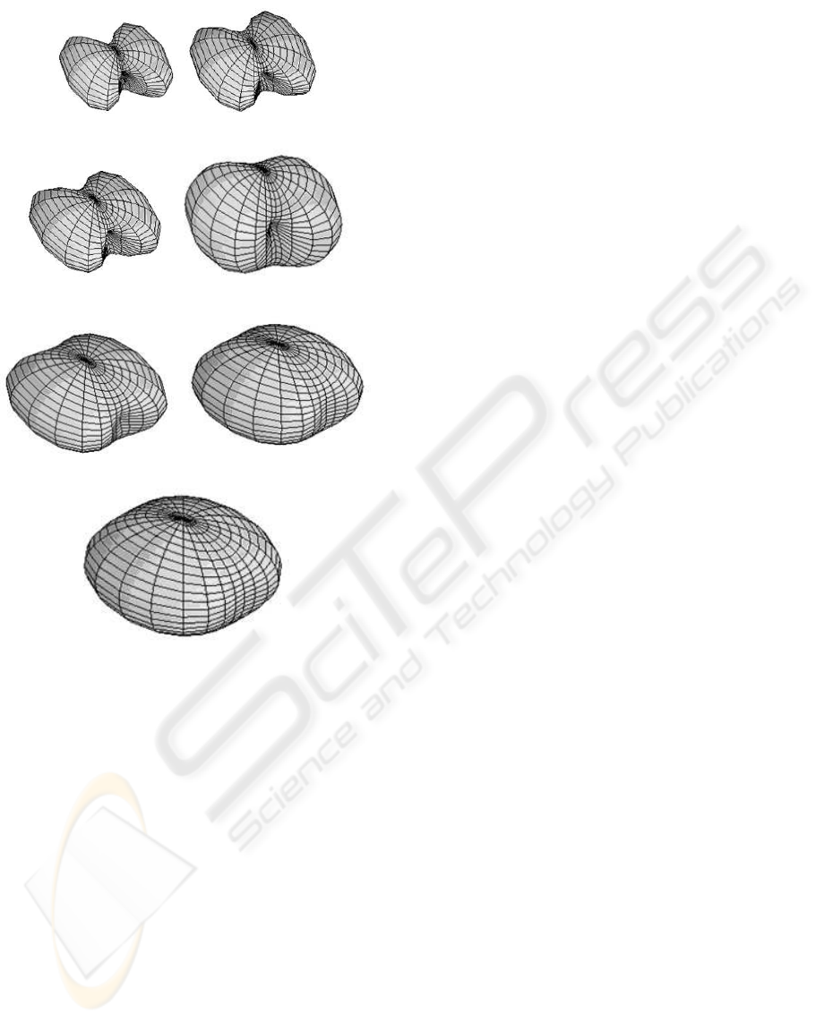
(a) (b)
(c) (d)
(e) (g)
(h)
Figure 11: Evolution of surface S with inflation process.
Size of S grows up and its curvature tends to 0 with time.
ACKNOWLEDGEMENTS
This work has been partially supported by a grant
of the Polytechnic University of Valencia, Spain
(”Programa de Apoyo a la Investigacion y Desar-
rollo 2006”), by the National Science Foundation un-
der grant CCF-0541032, by the MIUR-FIRB project
SHALOM under contract number RBIN04HWR8, by
the MIUR-PRIN project on ”Multi-resolution mod-
eling of scalar fields and digital shapes”, by the Eu-
ropean Network of Excellence AIM@SHAPE under
contract number 506766 and by the MCyT TIN2006-
15265-C06-04 Spanish project. We kindly thank Dr.
Fatiha M-Hammadi for the discussion we had on this
work.
REFERENCES
Ankerst, M. (2000). Visual Data Mining. PhD thesis,
Facultat fur Mathematik und Informatik der Lidwig-
Maximilians-Universitat Munchen.
Bajaj, C. L., Pascucci, V., and Shikore, D. R. (1998). Visu-
alization of scalar topology for structural enhacement.
In Proceedings of the IEEE Conference on Visualiza-
tion ’98 1998, pages 51–58.
Bajaj, C. L. and Shikore, D. R. (1998). Topology preserv-
ing data simplification with error bounds. Journal on
Computers and Graphics, 22(1):3–12.
Berger, M. and Gostiaux, B. (1972). G´emo´etrie
Diff´erentielle. Collection U.
Edelsbrunner, H., Harer, J., and Zomorodian, A. (2001).
Hierarchical morse complexes for piecewise linear 2-
manifolds. In Proc 17th Sympos. Comput. Geom.,
pages 70–79.
H. Edelsbrunner, J. Harer, V. N. V. P. (2003). Morse-smale
complexes for piecewise linear 3-manifolds. In Proc.
ACM Symposium on Computational Geometry, pages
361–370.
J.Toriwaki and Fukumura, T. (1975). Extraction of struc-
tural information from grey pictures. Computer
Graphics and Image Processing, 7:30–51.
Mangan, A. and Whitaker, R. (1999). Partitioning 3d
surface meshes using watershed. In IEEE Trans-
actionon visualization and Computer Graphics, vol-
ume 5, pages 308–321.
Massey, W. S. (1977). Algebraic Topology: an Introduction,
volume 56. Springer-Verlag.
Milnor, J. (1963). Morse Theory. Princeton University
Press.
Nackman, L. R. (1984). Two-dimensional critical point
configuration graph. IEEE Transactions on Pattern
Analysisand Machine Intelligence, PAMI-6(4):442–
450.
Peucker, T. K. and Douglas, E. G. (1975). Detection of
surface-specific points by local paprallel processing
of discrete terrain elevation data. Graphics Image
Processing, 4:475–387.
Smale, S. (1960). Morse inequalities for a dynamical
system. Bulletin of American Mathematical Society,
66:43–49.
Spivak, M. (1979). A comprehensive introduction to differ-
ential Geometry, volume 1. Houston, Texas.
Thom, R. (1949). Sur une partition en cellule associ´ees a
une fonction sur une vari´et´e. C.R.A.S., 228:973–975.
Vincent, L. and Soille, P. Watershed in digital spaces: an
efficient algorithm based on immersion simulation. In
IEEE Transactionon on Pattern Analysis and Machine
Intelligence, volume 13, pages 583–598.
Watson, L. T., Laffey, T. J., and Haralick, R. (1985). Topo-
graphic classification of digital image intensity sur-
faces using generalised splines and the discrete cosine
transformation. Computer Vision, Graphics and Im-
age Processing, 29:143–167.
THEORETICAL FOUNDATIONS OF 3D SCALAR FIELD VISUALIZATION
77