
AN ACTIVE STEREOSCOPIC SYSTEM FOR ITERATIVE 3D
SURFACE RECONSTRUCTION
Wanjing Li
Laboratory LE2i,University of Burgundy, Dijon, France
Laboratry i3Mainz, University of Applied Sciences, Mainz, Germany
Franck. S. Marzani, Yvon Voisin
Laboratory LE2i,University of Burgundy, Dijon, France
Frank Boochs
Laboratory i3Mainz, University of Applied Sciences, Mainz, Germany
Keywords: Active vision, 3D surface reconstruction, calibration, 3D triangular mesh, projector-camera system, adaptive
pattern projection, iterative reconstruction, surface curvature.
Abstract: For most traditional active 3D surface reconstruction methods, a common feature is that the object surface is
scanned uniformly, so that the final 3D model contains a very large number of points, which requires huge
storage space, and makes the transmission and visualization time-consuming. A post-process then is
necessary to reduce the data by decimation. In this paper, we present a newly active stereoscopic system
based on iterative spot pattern projection. The 3D surface reconstruction process begins with a regular spot
pattern, and then the pattern is modified progressively according to the object’s surface geometry. The
adaptation is controlled by the estimation of the local surface curvature of the actual reconstructed 3D
surface. The reconstructed 3D model is optimized: it retains all the morphological information about the
object with a minimal number of points. Therefore, it requires little storage space, and no further mesh
simplification is needed.
1 INTRODUCTION
In the field of 3D surface reconstruction and
metrology, including industrial applications,
stereoscopic systems are becoming increasingly
important. They can be divided into two categories:
passive or active (Battle et al., 1998; Horaud et al.,
1995).
In passive stereoscopic systems, cameras are
observing the object as it is without generating
optical information. Such systems use multiple
camera views to acquire the 3D object surface
information. In case of single camera systems, the
camera has to be moved to at least two known
positions around the object and takes images
sequentially at each position; in other cases, two or
more cameras being fixed in different positions take
images at the same time (Battle et al., 1998).
In active stereoscopic systems, a light projection
device is added to produce individual signals,
generate texture or code uniquely each surface
element (Battle et al., 1998). Individual signals
might be produced by a moving laser beam being
observed in a sequence of images; a certain texture
can be generated by projecting full-field light pattern
onto the object surface, so that each camera only
needs to take one image; for coded light approaches,
a projection sequence is necessary if the coding is
temporal, it is more sensitive to object appearance
and external light conditions (Krattenthaler et al.,
1994).
If we define respectively coordinate references
for the object (called “world reference”) and each
camera (called “camera reference”), the geometrical
relationship between the world reference and the
camera references can be described by extrinsic
parameters of the cameras, whereas the
78
Li W., S. Marzani F., Voisin Y. and Boochs F. (2007).
AN ACTIVE STEREOSCOPIC SYSTEM FOR ITERATIVE 3D SURFACE RECONSTRUCTION.
In Proceedings of the Second International Conference on Computer Vision Theory and Applications, pages 78-84
DOI: 10.5220/0002065500780084
Copyright
c
SciTePress
mathematical behavior of a camera is given by
intrinsic parameters. The intrinsic and extrinsic
parameters (that will be called “calibration
parameters” for simplification in the rest of the
paper) can be obtained respectively by camera
calibration and orientation process. Different
approaches were proposed (Faugeras et al., 1986;
Grün et al., 1992; Legarda-Saenz et al., 2004;
Marzani et al., 2002), and Garcia et al. (2000) made
a comparison of some approaches.
To determine the surface geometry of an object,
the 2D coordinates of a surface element in the
images are extracted respectively. If the calibration
parameters are known, the 3D coordinates of this
point in world reference can be calculated by
triangulation using all image rays to the object point.
In case of passive stereoscopic systems, image
rays are identified by using available texture on the
surface. For objects with low texture information,
the identification of the image rays becomes very
difficult; whereas in active systems, the projector
creates a synthetic texture on the surface of the
object, which simplifies the identification of image
rays, thus the rate of detected object points can be
highly increased.
For most of the previous pattern projection
methods, their common characteristic is the use of
pattern with a uniform resolution for the whole
object without considering the geometrical structure
of the surface. Such methods are necessary if the
object has complex surface geometry. However, for
those with relatively simple surface geometry, the
reconstructed 3D model can contain large number of
useless data which describes a plane area, and it can
easily reach to a size of gigabytes. The sheer amount
of data not only exhausts the main memory
resources of common desktop PCs, but also exceeds
the 4 gigabyte address space of 32-bit machines
(Isenburg et al., 2003); it makes the subsequent
processing difficult (ex., save, transmission,
rendering, etc.). Therefore, the further mesh
simplification is often necessary. However, it is
difficult to obtain an optimized model which retains
all morphological information about the object with
a minimum of points.
In this paper, we present a newly active
stereoscopic system based on an iterative projection
concept. The reconstruction process begins with a
regular spot pattern. After each iteration, the local
surface curvature of the actual reconstructed 3D
surface is estimated, and the density and distribution
of pattern spots are then modified for the next
iteration, thus the reconstructed 3D surface is refined
progressively. The final reconstructed 3D model was
proved to be optimized and needs much less storage
space compared to that obtained by traditional
solutions. This concept has been validated in
simulation working mode (Li et al., 2006). In this
paper, we focus on reality working mode.
The article is organized as follows: first, we
briefly present the 3D surface reconstruction system;
then we describe the following steps: system
calibration, initial pattern projection and iterative
process; finally, some reconstruction results are
given before we conclude and show perspectives.
2 SYSTEM DESCRIPTION
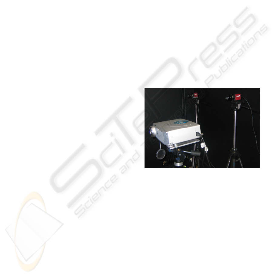
As shown in figure 1, the system consists of two
CCD cameras (Oscar F-510C, resolution:
2588x1958) and one LCD projector (Panasonic PT-
LB10E, resolution: 1024x768). A computer is
connected to them as the central control unit. It is
based on an iterative scheme (see figure 2), and is
controlled by a program developed in Matlab
language. A graphical interface is provided to user.
Figure 1: System setup.
Before the 3D reconstruction process begins, the
two cameras and the video projector should be
calibrated to obtain the calibration parameters. The
projector then projects initially a regular spot matrix
pattern onto the object. Each camera acquires an
image of the illuminated object. We extract the 2D
spot coordinates in the two images and then match
them. With the known calibration parameters, we
calculate the corresponding 3D object point
coordinates. A 3D surface mesh will then be
generated from the reconstructed 3D point cloud.
For each vertex of the 3D mesh, we estimate its
Gaussian curvature to decide if new spots should be
projected around it at next iteration. Finally, we
verify if the “condition of stop” is satisfied. If it is
the case, the process stops and the final
reconstructed 3D surface is obtained; otherwise, a
AN ACTIVE STEREOSCOPIC SYSTEM FOR ITERATIVE 3D SURFACE RECONSTRUCTION
79
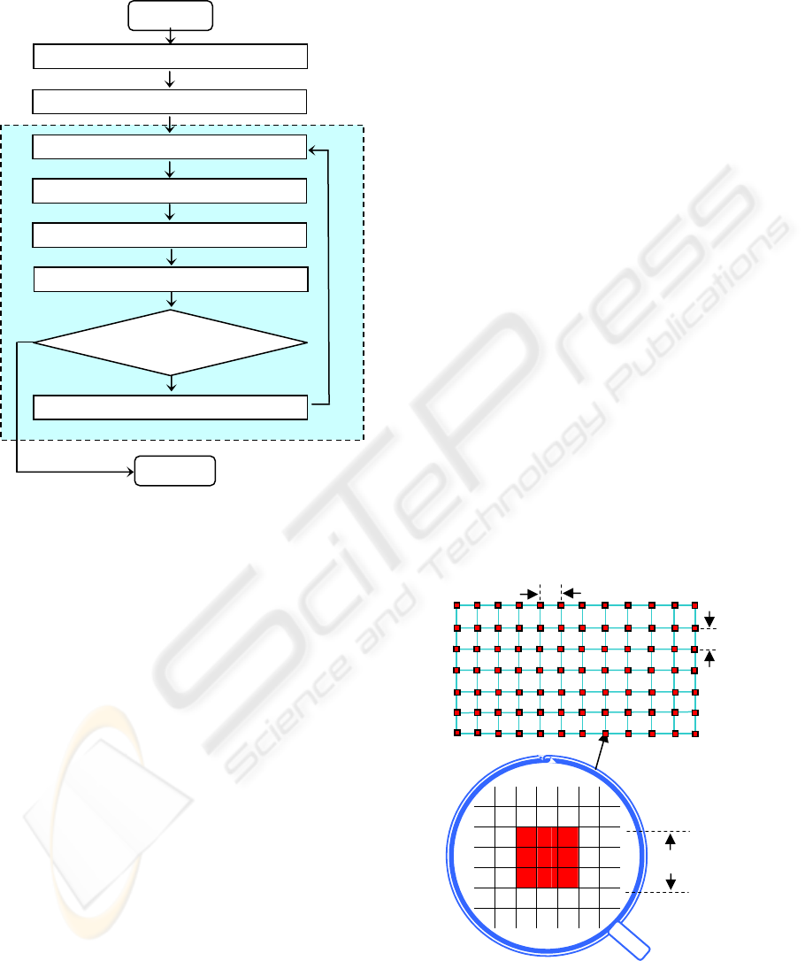
new pattern is generated, and the process goes back
to the image acquisition step and continues.
Figure 2: Iterative scheme.
In the following paragraphs, we describe how
the process works at each step. To simplify the
description, we suppose that P (u
,
v) is a pattern spot
and that V (x
,
y, z) is its representation on the object.
V can also be a vertex of current 3D triangular mesh
which approximates the object surface.
3 SYSTEM CALIBRATION
The calibration of the two cameras and the video
projector is indispensable. Actually, in our system,
the calculation of 3D point coordinates is based on
the images acquired by the two cameras. Therefore
we need to know the calibration parameters of the
two cameras; those of the projector have also to be
known for new pattern generation (see 5.6).
CCD camera and LCD projector can both be
described by a geometrical model called “pinhole”
(Lathuilière et al., 2003). In such a model, the
extrinsic parameters are the rotation matrix R and
the translation matrix T; these two matrices describe
the geometrical relationship between the world
reference and the camera/projector reference (Tsai,
1986). The intrinsic parameters are:
f : the focal length;
O (u
0
, v
0
) : the intersection point between the
image plan and the optical axis of the camera;
k
u
: the vertical scale factor (pixels/mm) in
image plan;
k
v
: the horizontal scale factor.
To get all these parameters, the system is
calibrated in two steps by applying Faugeras-
Toscani approach (Faugeras et al., 1986). At the first
step, a calibration target is used to obtain the
calibration parameters of the two cameras without
using the video projector. At the second step, the
projector projects a certain spot pattern onto the
object. Each camera then acquires an image of the
object. By using the calibration parameters of the
two cameras obtained at the first step, we can
calculate the 3D coordinates of the object points
from the image points, so that the calibration
parameters of the video projector can be obtained
from the projected 2D pattern points and the
reconstructed 3D object points.
4 INITIAL PATTERN
The initial pattern is defined by 4 values (in pixels):
(u
1
, v
1
): upper left point coordinates;
(u
2
, v
2
): down right point coordinates;
s: spot size;
d
0
: distance between two adjacent spots.
Figure 3: Definition of the initial pattern.
s = 3 pixels
(u
2
, v
2
)
(u
1
, v
1
)
d
0
d
0
3D surface mesh generation
Yes
N
o
System calibration
N
ew pattern generation and projection
“Condition of stop”
satisfied?
END
BEGIN
Initial pattern
p
rojection
Image acquisition
3D point cloud reconstruction
Local surface curvature estimation
Iterative process
VISAPP 2007 - International Conference on Computer Vision Theory and Applications
80
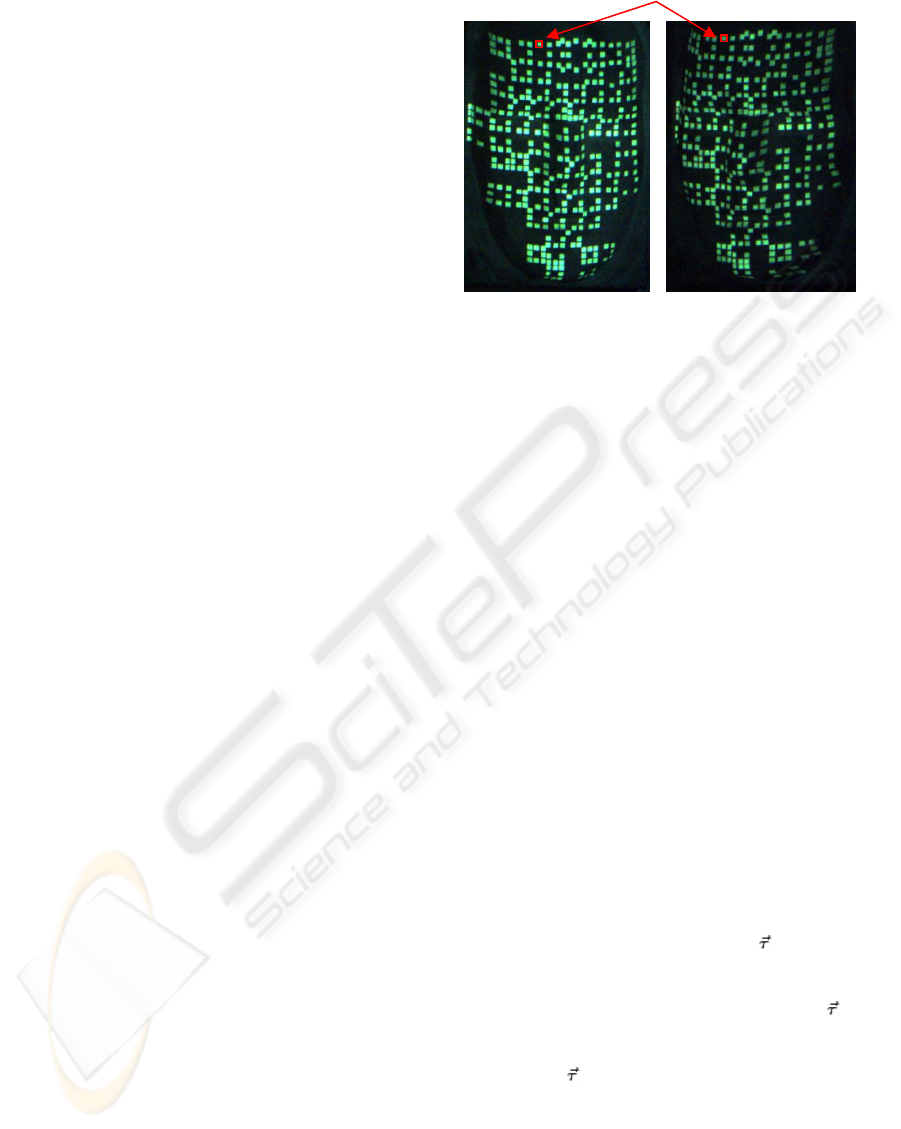
Figure 3 illustrates how the initial pattern is
defined by these values. The definition of initial
pattern is quite important. If the object has some
small surface variations, the spots should be dense
enough to cover all these small areas. Otherwise, the
reconstructed initial 3D surface might be flat in
these areas. In consequence, at the next iteration, no
pattern spot would be projected around these areas
since its local surface curvature is not strong enough.
As a result, the final reconstructed 3D model might
lose partially geometrical information.
5 ITERATIVE PROCESS
5.1 Image Acquisition
Once the pattern is projected, each camera takes an
image of the illuminated object. These two images
are saved in the memory for 3D point cloud
reconstruction.
5.2 3D Point Cloud Reconstruction
The process of 3D point cloud reconstruction can be
divided into 3 steps:
2D image point detection;
2D image point matching;
3D object point coordinates calculation.
To detect image points, we first apply several
image processing techniques, such as filtering,
thresholding, and contour recognition, to get the
boundary of the spot. Then, all pixels within the
boundary are considered for a weighted calculation
of the center of gravity, which gives the center of the
image ray.
The correspondence problem then should be
resolved, i.e., to identify, for a given point in one
image, its correspondence in the other one (see
figure 4). Since the images are calibrated and
oriented in space, we can simplify the
correspondence problem by applying some
geometrical constraints. The most important one is
based on the fact that corresponding points are
imaged on epipolar lines. Some other constraints
come from the relative position of two adjacent
object points, or the probability of having major
changes in the distance from the image to object
(Böhler et al., 2006).
Finally, for each pair of matched image points,
by using the calibration parameters for each camera,
we calculate, by ray intersection, the 3D coordinates
of the corresponding object point.
(a) (b)
Figure 4: An example of acquired images, (a) Image
acquired by left camera, (b) Image acquired by right
camera.
5.3 Mesh Generation
Once the 3D point cloud is obtained, we generate a
3D surface mesh by Delaunay triangulation. The
Delaunay triangulation is generally unique. It has the
property that the outcircle of every triangle does not
contain any other point. The Delaunay triangulation
is the dual structure of the Voronoi diagram
(Kanaganathan et al., 1991).
5.4 Surface Curvature Estimation
From a theoretical point of view, triangular meshes
do not have any curvature at all, since all faces are
flat and the curvature is not properly defined along
edges and at vertices because the surface is not C
2
-
differentiable. However, thinking of a triangular
mesh as a piecewise linear approximation of an
unknown smooth surface, the curvature of that
unknown surface might be calculated using the
information given by the triangular mesh itself (Dyn
et al., 2001). A normal curvature is the
generalization of surface curvatures. Given a point P
on the surface S and a direction
lying in the
tangent plane of the surface S at P, the normal
curvature is calculated by intersecting S with the
plane spanned by P, the normal to S at P, and
. The
normal curvature is the signed curvature of this
curve at P. If we compute the normal curvature for
all values of
in the tangent plane at P, we will get
a maximum value k
1
and a minimum value k
2
in two
orthogonal directions. k
1
and k
2
are called principal
curvatures.
The Gaussian curvature K (also called total
curvature) and mean curvature H are differential
invariant properties which depend only upon the
surface’s intrinsic geometry, and play a very
Same object point
AN ACTIVE STEREOSCOPIC SYSTEM FOR ITERATIVE 3D SURFACE RECONSTRUCTION
81
important role in the theory of surfaces. They are
defined as follow:
K = k
1
× k
2
, (1)
H = (k
1
+ k
2
) / 2. (2)
In our work, we chose the Gaussian curvature to
evaluate the local surface curvature, since for a
minimal surface, the mean curvature is zero
everywhere, whereas Gaussian curvature may vary
in different zones; besides, the sign of Gaussian
curvature gives extra information about the type of
the local piecewise surface. A positive Gaussian
curvature value means the surface is locally either a
peak or a valley. A negative value means the surface
locally has a saddle. And a zero value means the
surface is flat in at least one direction (i.e., both a
plane and a cylinder have zero Gaussian curvature)
(Alboul et al., 2005).
As we can see, the Gaussian curvature and mean
curvature are defined only for twice differentiable
(C
2
) surfaces. To get 3D surface curvature
information, different approaches have been
proposed to estimate Gaussian and mean curvature
(Alboul et al., 2005; Surazhsky et al., 2003; Peng et
al., 2003). Surazhsky et al. (2003) compared five
curvature estimation algorithms, and drew a
conclusion that the Gauss-Bonnet scheme is the best
algorithm for the estimation of Gaussian curvature.
We therefore estimate the curvature as follows:
Vertex V
i
is considered as a neighbor of vertex V
if the edge
belongs to the mesh. Denote the set
of neighbors of V by {V
i
| i =1, 2, ..., n}, the set of
triangles containing V by {T
i
= Δ (V
i
, V, V
(i+1)
mod n
) |
i =1, 2, ..., n}, and the set of angles between V and
its two successive neighbors by {
= (V
i
, V, V
(i+1)
mod n
) | i =1, 2, ..., n} (see figure 5-(a)). According to
the Gauss-Bonnet scheme (Surazhsky et al., 2003),
the Gaussian curvature K at vertex V is estimated as
(3)
where A is the
sum of the areas of triangles T
i
around the vertex V.
This estimation method works well when vertex
V is close enough to its neighbors. Obviously, it is
not our case, since we start from a rough 3D surface
mesh and refine it progressively. In (Alboul et al.,
2005), Alboul et al. indicated that we can ignore A
and simply estimate the Gaussian curvature K at
vertex V as in (4):
5.5 “Condition of Stop” Verification
At the end of each iteration, the condition of stop is
verified by the following algorithm:
Target = {};
For each vertex V of current mesh
K = Gaussian curvature of V
If K < t
c1
Delete V from the mesh;
Else if K > t
c2
d = average distance between V
and all its neighbors;
If d > t
d
Target = Target + {V};
End
End
End
If Target == {}
Process stops;
Else
Generate new pattern;
End
where t
c1
is the pre-defined threshold for “weak
curvature”; t
c2
is the threshold for “strong curvature”;
and t
d
is the threshold for “minimal average distance
to neighbors”. Actually, in some cases, even after a
great number of iterations, the local surface
curvature K of V is always much higher than t
c2
.
Therefore, to avoid infinite iteration, we introduced
the threshold t
d
.
5.6 New Pattern Generation
To generate the new pattern, firstly, for each target
vertex V obtained at previous step, if it has “closed”
neighborhood (see figure 5), we calculate the 2D
coordinates of its corresponding pattern spot P by
using the calibration parameters of the video
projector. Then eight new spots are added around it
in the new pattern. A single value d is enough to
specify their positions (see figure 6).
(a) (b)
Figure 5: Different types of vertex neighborhood in 3D
triangular mesh: (a) “closed” neighborhood, (b) not
“closed” neighborhood.
(
4
)
VISAPP 2007 - International Conference on Computer Vision Theory and Applications
82
d
v
u
d
Figure 6: New pattern generation from a target pattern
spot.
Since the density of the 3D triangular mesh
increases after each iteration, the value of d has to be
adapted to the current 3D mesh. We therefore set the
value of d according to the average distance D
between the vertex V and all its neighbors in the
current 3D mesh as: d = r×D, where r is a ratio pre-
configured by user, it can be ½, ¼, or
1
/
9
, etc.
“Old” pattern spots will not be added into new
patterns because their reconstruction has already be
done. However, we keep the 3D point cloud
obtained at each iteration, so that they can be used
for 3D mesh generation at next iteration, thus the 3D
model is refined progressively.
Finally, we optimize the generated new pattern by
deleting those spots which are too close to each
other, so that at the next iteration, the 2D image
point detection and the 2D point matching will be
simplified.
6 RESULTS
We tested our system on several real objects. In this
paper, we show the reconstruction results of a mask,
since it has partial complex surface curvature. The
size of the mask is 150 mm (l) × 200 mm (h) ×130
mm (w). Figure 7 shows an example of
reconstruction results for the mask. In this example,
t
c1
= 0.001, t
c2
= 0.04, t
d
= 5 mm, r =
1
/
3
. The initial
pattern was defined as follows:
(u
1
, v
1
) = (100,100);
(u
2
, v
2
) = (700,760);
s = 3 pixels;
d
0
= 25 pixels.
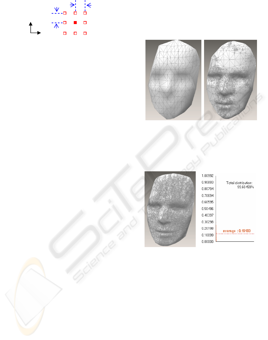
To evaluate the quality of the reconstructed 3D
surface by our system, we scanned the mask by
using a traditional method, i.e. by projecting a
vertical stripe and shifting it from left to right, pixel
by pixel, the 3D surface obtained contains 10177
points. We then compared it to the one obtained by
our system by calculating the distance error, it
showed that the error in distance is very slight: The
average error is only 0.19 mm; and the maximal
error is 0.32mm (see figure 8). Besides, we can see
that the 3D surface obtained by traditional method
contains 10177 points, whereas the one obtained by
our system contains only 770 points, which means
that the number of points of the 3D surface was
reduced more than 90%.
(a) (b)
Figure 7: Reconstructed 3D surface of the mask, (a) initial
3D surface - 152 points, (b) Final 3D surface - 770 points.
(a) (b)
Figure 8: (a) 3D surface obtained by traditional method -
10177 points, (b) distance error between the 3D surface
reconstructed by using our approach and the one issued
from traditional method.
7 CONCLUSIONS
We presented an adapted 3D surface reconstruction
approach based on active vision system. The concept
is to restrict data capture to characteristic surface
parts during the image acquisition process, thus the
reconstructed 3D model will be ensured to be fitted
to the morphology of an object. The system projects
iteratively spot patterns adapted to the object surface
geometry. At each iteration, we calculate the local
AN ACTIVE STEREOSCOPIC SYSTEM FOR ITERATIVE 3D SURFACE RECONSTRUCTION
83

surface curvature for each vertex of the actual 3D
mesh and decide where to project more points.
This approach was proved to be very efficient,
because the reconstructed 3D surface needs much
less storage space compared to that obtained by
traditional method and does not need a post-process
for decimation. The quality of reconstructed 3D
surface is very satisfactory: compared to the one
issued from traditional method, the 3D surface of the
mask obtained by applying our approach has an
average distance error of less than 0.2 mm. The
whole reconstruction process takes only several
minutes. Compared to the traditional method, our
system is not faster. However, the later time-
consuming mesh simplification procedure can be
avoided since the 3D model obtained is optimized.
Our future work will focus on the improvement
of the system. Special efforts will be made on image
processing, surface curvature estimation and the
generation of new patterns. Once the system
becomes robust, we hope to apply this 3D
reconstruction approach to industrial application,
such as quality control, etc.
ACKNOWLEDGEMENTS
The authors gratefully acknowledge the support of
European Social Funds (France), University of
Applied Sciences in Mainz (Germany), and Regional
Council of Burgundy (France).
REFERENCES
Alboul, L., Echeverria G., Rodrigues, M., 2005. Discrete
curvatures and gauss maps for polyhedral surfaces, in
European Workshop on Computational Geometry
(EWCG), Eindhoven, the Netherlands, pp. 69–72.
Battle, J., Mouaddib, E., Salvi, J., 1998. Recent progress
in coded structured light as a technique to solve the
correspondence Problem: a Survey, Pattern
Recognition, 31(7), pp. 963-982.
Böhler, M., Boochs, F., 2006. Getting 3D shapes by means
of projection and photogrammetry, Inspect, GIT-
Verlag, Darmstadt.
Dyn, N., Hormann, K., Kim S. J., Levin, D., 2001.
Optimizing 3D triangulations using discrete curvature
analysis, Mathematical Methods for Curves and
Surfaces, Oslo 2000, Nashville, TN, pp.135-146.
Faugeras, O. D., Toscani, G., 1986. The calibration
problem for stereo, in Proc. Computer Vision and
Pattern Recognition, Miami Beach, Florida, USA,
pp.15-20.
Garcia, D., Orteu, J.J., Devy, M., 2000. Accurate
Calibration of a Stereovision Sensor: Comparison of
Different Approaches, 5th Workshop on Vision
Modeling and Visualization (VMV'2000), Saarbrücken,
Germany, pp.25-32.
Grün, A., Beyer, H., 1992. System calibration through
self-calibration, Workshop on Calibration and
Orientation of Cameras in Computer Vision,
Washington D.C..
Horaud, R., Monga, O., 1995. Vision par ordinateur:
outils fondamentaux, Hermès, 2
nd
edition.
Isenburg, M., Lindstrom, P., Gumhold, S., Snoeyink, J.,
2003. Large mesh simplification using processing
sequences, in Proc. Visualization'03, pp. 465-472.
Kanaganathan, S., Goldstein, N.B., 1991. Comparison of
four point adding algorithms for Delaunay type three
dimensional mesh generators, IEEE Transactions on
magnetics, 27(3).
Krattenthaler, W., Mayer, K.J., Duwe, H.P., 1994. 3D-
surface measurement with coded light approach, In
Proc. of the 17th meeting of the Austrian Association
for Pattern Recognition on Image Analysis and
Synthesis, pp. 103-114.
Lathuilière, A., Marzani, F., Voisin, Y., 2003. Calibration
of a LCD projector with pinhole model in active
stereovision applications. Conference SPIE :Two- and
Three-Dimensional Vision Systems for Inspection,
Control, and Metrology, Rhode Island, USA, 5265,
pp. 199-204.
Legarda-Saenz, R., Bothe, T., Jüptner, W.P., 2004.
Accurate Procedure for the Calibration of a Structured
Light System, Optical Engineering, 43(2), pp.464-
471.
Li, W., Boochs, F., Marzani, F., Voisin, Y., 2006.
Iterative 3D surface reconstruction with adaptive
Pattern projection, in Proc. of the Sixth IASTED
International Conference on Visulatization, Imaging
and Image Processing (VIIP), Palma De
Mallorca, Spain, pp.336-341.
Marzani, F., Voisin, Y., Diou, A., Lew Yan Voon, L.F.C.,
2002. Calibration of a 3D reconstruction system using
a structured light source, Journal of Optical
Engineering, 41 (2), pp. 484-492.
Peng, J., Li, Q., Jay kuo C.C., Zhou, M., 2003. Estimating
Gaussian Curvatures from 3D meshes. SPIE
Electronic Image, vol.5007, pp. 270-280.
Surazhsky, T., Magid, E., Soldea, O., Elber, G., Rivlin, E.,
2003. A comparison of gaussian and mean curvatures
estimation methods on triangular meshes, in IEEE
International Conference on Robotics & Automation.
Tsai, R.Y., 1986. An efficient and accurate camera
calibration technique for 3D machine vision, IEEE
Computer Vision and Pattern Recognition, Miami
Beach Florida, pp.364-374.
VISAPP 2007 - International Conference on Computer Vision Theory and Applications
84
