
VARIATIONAL POSTERIOR DISTRIBUTION APPROXIMATION IN
BAYESIAN EMISSION TOMOGRAPHY RECONSTRUCTION USING
A GAMMA MIXTURE PRIOR
Rafael Molina
1
, Antonio L´opez
2
, Jos´e Manuel Mart´ın
1
and Aggelos K. Katsaggelos
3
1
Departamento de Ciencias de la Computaci´on e I.A., Universidad de Granada, 18071 Granada, Spain
2
Departamento de Lenguajes y Sistemas Inform´aticos, Universidad de Granada, 18071 Granada, Spain
3
Department of Electrical Engineering and Computer Science, Northwestern University, Evanston, Illinois 60208-3118
Keywords:
Image reconstruction, parameter estimation, Bayesian framework, variational methods, Tomography images.
Abstract:
Following the Bayesian framework we propose a method to reconstruct emission tomography images which
uses gamma mixture prior and variational methods to approximate the posterior distribution of the unknown
parameters and image instead of estimating them by using the Evidence Analysis or alternating between the
estimation of parameters and image (Iterated Conditional Mode (ICM)) approach. By analyzing the posterior
distribution approximation we can examine the quality of the proposed estimates. The method is tested on real
Single Positron Emission Tomography (SPECT) images.
1 INTRODUCTION
SPECT (Single Photon Emission Computed Tomog-
raphy) and PET (Positron Emission Tomography) are
non invasive techniques which are used in Nuclear
Medicine to take views of a isotope distribution in
an patient. Since SPECT and PET obtain images
via emission mode, both techniques are referred to as
emission tomography.
In this paper, we address the problem of the re-
construction of emission tomography images. We
propose the use of the hierarchical Bayesian frame-
work to incorporate knowledge on the expected char-
acteristics of the original image in the form of a mix-
ture of gamma distributions, to model the observa-
tion process, and also to include information on the
unknown parameters in the model in the form of hy-
perprior distributions. Then, by applying variational
methods to approximate probability distributions we
estimate the unknown parameters and the underlying
original image.
The paper is organized as follows. In section 2
the Bayesian modeling and inference for our problem
is presented. The used probability distributions for
emission tomography images are formulated in sec-
tion 3. The Bayesian analysis and posterior proba-
bility approximation to obtain the parameters and the
original image is performed in section 4. The applica-
tion of this method to a real SPECT study is described
in section 5 and, finally, section 6 concludes the paper.
2 BAYESIAN FORMULATION
Let the object to be estimated be represented by a
vector x of N lexicographically ordered voxels x =
{x
1
,... ,x
N
}. The observed, noisy data from which x
is to be estimated is given by the vector y, comprising
lexicographically ordered elements y = {y
1
,... ,y
M
},
where M is the number of detectors in the tomography
system.
The Bayesian formulation of the Nuclear Medi-
cine image reconstruction problem requires the def-
inition of the joint distribution p(Ω,x,y) of the ob-
servation y, the unknown original image x, and the
hyperparameters Ω, describing their distributions.
To model the joint distribution we utilize the
hierarchical Bayesian paradigm (see, for example
(Molina et al., 1999; Galatsanos et al., 2002)). In
the hierarchical approach we have two stages. In the
first stage, knowledge about the structural form of the
165
Molina R., López A., Manuel Martín J. and K. Katsaggelos A. (2007).
VARIATIONAL POSTERIOR DISTRIBUTION APPROXIMATION IN BAYESIAN EMISSION TOMOGRAPHY RECONSTRUCTION USING A GAMMA
MIXTURE PRIOR.
In Proceedings of the Second Inter national Conference on Computer Vision Theory and Applications, pages 165-173
DOI: 10.5220/0002066001650173
Copyright
c
SciTePress

observation noise and the structural behavior of the
underlying image is used in forming p(y | x,Ω) and
p(x | Ω), respectively. In the second stage a hyper-
prior on the hyperparameters is defined, thus allowing
the incorporation of information about these hyperpa-
rameters into the process.
Then the following joint distribution is defined for
Ω, x, and y,
p(Ω,x,y) = p(Ω)p(x | Ω)p(y | x,Ω), (1)
and inference is based on p(Ω,x | y) (see
(Mohammad-Djafari, 1995), (Mohammad-Djafari,
1996)).
We can alternate the maximization of p(Ω,x | y)
with respect to Ω and x (the ICM approach), (Hsiao
et al., 2002). However, this alternative maximization
does not take into account the uncertainty in the orig-
inal image when estimating the unknown parameters
of the model and the consequential effect on the esti-
mation of these parameters. An alternative methodol-
ogy consists of estimating the hyperparameters in Ω
by using
ˆ
Ω = argmax
Ω
p(Ω | y) = argmax
Ω
x
p(Ω,x,y)dx, (2)
and then estimating the original image by solving
ˆ
x = argmax
x
p(x |
ˆ
Ω,y). (3)
This inference procedure (called Evidence Analysis)
aims at optimizing a given function and not at obtain-
ing a posterior distribution that can be simulated to
obtain additional information on the quality of the es-
timates.
The calculation of p(Ω, x | y), however, may not
be possible, in which case we have to decide how to
approximateit. The Laplace approximation of distrib-
utions has been used, for instance, in blind deconvolu-
tion problemswhen the blur is partially known(Galat-
sanos et al., 2002; Galatsanos et al., 2000). An alter-
native method is provided by variational distribution
approximation. This approximation can be thought
of as being between the Laplace approximation and
sampling methods (Andrieu et al., 2003). The basic
underlying idea is to approximate p(Ω,x | y) with a
simpler distribution, usually one which assumes that
x and the hyperparameters are independent given the
data (see chapter II in (Beal, 2003) for an excellent
introduction to variational methods and their relation-
ships to other inference approaches).
The last few years have seen a growing inter-
est in the application of variational methods (Likas
and Galatsanos, 2004; Miskin, 2000; Molina et al.,
2006) to inference problems. These methods attempt
to approximate posterior distributions with the use of
the Kullback-Leibler cross-entropy (Kullback, 1959).
Application of variational methods to Bayesian infer-
ence problems include graphical models and neuronal
networks (Jordan et al., 1998), independent compo-
nent analysis (Miskin, 2000), mixture of factor ana-
lyzers, linear dynamic systems, hidden Markov mod-
els (Beal, 2003), support vector machines (Bishop
and Tipping, 2000) and blind deconvolution problems
(Miskin and MacKay, 2000; Likas and Galatsanos,
2004; Molina et al., 2006).
3 HYPERPRIORS, PRIORS AND
OBSERVATION MODELS
For emission tomography the conditional distribution
of the observed data y given x has the form
p(y | x) ∝
M
∏
i=1
exp{−
N
∑
j=1
A
i, j
x
j
}(
N
∑
j=1
A
i, j
x
j
)
y
i
, (4)
where A
i, j
is the contribution of the jth element of x
to the ith element of y. The system matrix A, with
elements A
i, j
, i = 1,...,M, j = 1, ..., N depends on
the geometry of the gamma camera and effects, such
as, the photon attenuation and the scatter contribution.
This model together with the image model constitute
the first stage of the hierarchical Bayesian modeling.
For the image to be estimated we use as prior
model
p(x | π,β, α) =
N
∏
j=1
C
∑
c=1
π
c
p
G
(x
j
| β
c
,α
c
)
!
, (5)
where, for a given number of classes C, π denotes the
C-dimensional vector π = (π
1
,... ,π
C
) consisting ofC
mixing proportions (weights) which are positive and
satisfy the normalization constraint
C
∑
c=1
π
c
= 1, (6)
and α and β denote, respectively, the C-dimensional
vectors α = (α
1
,... ,α
C
), β = (β
1
,...,β
C
) satisfying
α
c
> 1 and β
c
> 0, ∀c. Each pair (α
c
,β
c
) defines for
x > 0 the gamma probability distribution
p
G
(x | β
c
,α
c
) =
α
c
β
c
α
c
1
Γ(α
c
)
x
α
c
−1
e
−(α
c
/β
c
)x
. (7)
The mean, variance, and mode of this gamma dis-
tribution are given by
E[x] = β
c
Var[x] = β
2
c
/α
c
Mode[x] = β
c
(1− 1/α
c
).
(8)
The parameter β
c
plays the role of the mean of
cluster c while the pair β
c
, α
c
controls the variance of
VISAPP 2007 - International Conference on Computer Vision Theory and Applications
166

the prior distribution. There are then two nice inter-
pretations of the parameter α
c
it controls the smooth-
ness of the reconstruction in class c and also mea-
sures the confidence on the prior mean. This second
interpretation resembles the confidence values on the
hyperprior parameters in image restoration problems
(see, for instance, (Molina et al., 1999; Galatsanos
et al., 2000; Galatsanos et al., 2002)). In this pa-
per, following the approach in (Hsiao et al., 2002) we
will not attempt to estimate α
c
and leave it as an user-
specified parameter.
The use of gamma priors in medical images was
introduced in (Lange et al., 1987). To our knowledge
the use of mixtures of gamma priors in medical imag-
ing was first proposed in (Hsiao et al., 1998) for trans-
mission tomography.
We now proceed to introduce the prior distribution
(hyperprior) on the unknown parameters. We note
that the set of unknown parameters is given by
Ω =
n
ω = (π,β) = (π
1
,...,π
C
,β
1
,... ,β
C
) |
π
c
≥ 0 ∀c with
∑
c
π
c
= 1, and β
c
> 0,∀c
o
.(9)
Following the Bayesian paradigm we have to de-
fine now the hyperprior distribution on Ω. We can use
the following distribution on the unknown hyperpara-
meters ω ∈ Ω,
p(ω) = p(π)p(β), (10)
where p(π) and p(β) are flat (assigning the same prob-
ability to all elements) distributions. We can, how-
ever, include additional information on the mixing
weights by using as p(π) the C-variate Dirichlet dis-
tribution defined by
p(π) = p(π
1
,... ,π
C
)
=
Γ(a
1
+ ·· · + a
C
)
Γ(a
1
)··· Γ(a
C
)
π
a
1
−1
1
···π
a
C
−1
C
, (11)
over π
c
≥ 0 ∀c, with
∑
c
π
c
= 1 and zero outside,
where the a
c
’s are all real and positive. We will re-
fer to a distribution having the density function given
in equation (11) as the C-variate Dirichlet distribu-
tion D(a
1
,... ,a
C
). A D(a
1
,... ,a
C
) distribution has
the following marginal means and variances,
E[π
c
] =
a
c
a
1
+ ·· · + a
C
Var[π
c
] =
a
c
(a
1
+ ·· · + a
C
− a
c
)
(a
1
+ ·· · + a
C
)
2
(a
1
+ ·· · + a
C
+ 1)
,
c = 1, ...,C, (12)
(see (Wilks, 1962)). Note that if a
c
= ρl
c
, where
l
c
> 0, ∀c and ρ > 0, the mean of π
c
does not depend
on ρ, while ρ can be used to increase or decrease the
variance of π
c
.
We will assume that β
c
, c = 1, ...,C has as hyper-
prior distribution p(β
c
), the inverse gamma distribu-
tion defined by
p
IG
(β
c
| m
0
c
,n
0
c
) =
((m
0
c
− 1)n
0
c
)
m
0
c
Γ(m
0
c
)
×
β
−m
0
c
−1
c
e
−(m
0
c
−1)n
0
c
/β
c
. (13)
where m
0
c
> 1 and n
0
c
> 0, ∀c, and the mean, variance,
and mode of this inverse gamma distribution are given
by
E[β
c
] = n
0
c
, Var[β
c
] = (n
0
c
)
2
/(m
0
c
− 2),
Mode[β
c
] = (m
0
c
− 1)n
0
c
/(m
0
c
+ 1). (14)
We now have a probability distribution defined
over (π,β,x, y) which has the form
p(π,β,x,y) = p(π)p(β)p(x | π,β)p(y | x) (15)
4 BAYESIAN INFERENCE AND
VARIATIONAL
APPROXIMATION
In order to perform inference we need to either
calculate or approximate the posterior distribution
p(π,β,x | y). Since this posterior distribution can not
be found in closed form, we will apply variational
methods to approximate this distribution by the dis-
tribution q(π,β,x).
The variational criterion used to find q(π,β,x)
is the minimization of the Kullback-Leibler diver-
gence, given by (Kullback and Leibler, 1951; Kull-
back, 1959)
C
KL
(q(π,β,x) k p(π,β,x | y)) =
=
π,β,x
q(π,β,x)log
q(π,β,x)
p(π,β,x | y)
dπdβdx
=
π,β,x
q(π,β,x)log
q(π,β,x)
p(π,β,x,y)
dπdβdx
+logp(y), (16)
which is always non negative and equal to zero only
when q(π,β, x) = p(π,β,x | y).
We choose to approximate the posterior distribu-
tion p(π,β,x | y) by the distribution
q(π,β,x) = q(π)q(β)q(x), (17)
where q(π), q(β) and q(x) denote distributions on π,
β and x respectively. In the following we provide the
derivation of two approximations of the posterior dis-
tribution as well as their algorithmic descriptions.
VARIATIONAL POSTERIOR DISTRIBUTION APPROXIMATION IN BAYESIAN EMISSION TOMOGRAPHY
RECONSTRUCTION USING A GAMMA MIXTURE PRIOR
167

4.1 General Case
We now proceed to find the best of these distributions
in the divergence sense.
Let
Φ = {π, β,x}. (18)
For θ ∈ Φ let us denote by Φ
θ
the subset of Φ with
θ removed; for instance, if θ = x, Φ
x
= (π,β). Then,
Eq. (16) can be written as
C
KL
(q(π,β,x) k p(π,β,x | y))
= C
KL
(q(θ)q(Φ
θ
) k p(π,β,x | y))
=
θ
q(θ)
Φ
θ
q(Φ
θ
)log
q(θ)q(Φ
θ
)
p(π,β,x,y)
dΦ
θ
dθ
+const. (19)
Now, given q(Φ
θ
) =
∏
ρ6=θ
q(ρ), (if, for instance,
θ = x then q(Φ
x
) = q(π)q(β)), an estimate of q(θ) is
obtained as
ˆq(θ)=argmin
q(θ)
C
KL
(q(θ)q(Φ
θ
)) k p(π,β, x | y)).
(20)
Thus, we have the following iterative procedure
to find q(π,β,x).
Algorithm 1 General case. Iterative estimation of
q(π,β,x) = q(π)q(β)q(x).
Given q
1
(β), and q
1
(x), the initial estimates of the
distributions q(β), and q(x),
For k = 1,2,... until a stopping criterion is met:
1. Find
q
k
(π) =
argmin
q(π)
C
KL
(q(π)q
k
(β)q
k
(x) k p(π, β,x | y)), (21)
2. Find
q
k+1
(β) =
argmin
q(β)
C
KL
(q
k
(π)q(β)q
k
(x) k p(π, β,x | y)), (22)
3. Find
q
k+1
(x) =
argmin
q(x)
C
KL
(q
k
(π)q
k+1
(β)q(x)kp(π,β,x| y))(23)
Set
q(π)= lim
k→∞
q
k
(π), q(β)= lim
k→∞
q
k
(β), q(x)= lim
k→∞
q
k
(x).
(24)
4.2 Degenerate Case
In the previous algorithm we have performed the
search of the distributions q(π), q(β), and q(x) in
an unrestricted manner. However, we can reduce the
space of search to the set of degenerate distributions.
This approach, to be developed now, will not provide
information on the quality of the estimates but we use
it to justify some of the estimation procedures pro-
posed in the literature as the solution of the variational
approach to posterior distributions when a particular
distribution approximation is used.
Let
A =
π=(π
1
,... ,π
C
) | π
c
≥ 0 ∀c with
∑
c
π
c
=1
.
(25)
and
B = {β = (β
1
,... ,β
C
) | β
c
> 0 ∀c }. (26)
Instead of using an unrestricted search for the distrib-
ution of q(π), q(β), and q(x) we will here restrict our
search to the following sets of distributions
D(A) = {q(π) | q(π) is a degenerate
distribution on an element of A} (27)
D(B) = {q(β) | q(β) is a degenerate
distribution on an element of B} (28)
D((R
+
0
)
N
) = {q(x) | q(x) is a degenerate
distribution on an element of (R
+
0
)
N
},(29)
where a degenerate distribution takes one value with
probability one, that is,
q(θ) =
1 if θ = θ
0 otherwise
(30)
When q
k
(π), q
k
(β), and q
k
(x) are degenerate dis-
tributions, we will denote by π
k
, β
k
, and x
k
respec-
tively the values these distributions take with proba-
bility one. We will also use the subscript D on the
distributions q(·) to denote the degenerate approxi-
mations q
D
(·). Then, the variational approach when
using degenerate distributions becomes:
Algorithm 2 Degenerate case. Iterative estimation
of q
D
(π,β,x) = q
D
(π)q
D
(β)q
D
(x)
Given β
1
∈ B, and x
1
, the initial estimates of β and x,
respectively, for k = 1,2,. . . until a stopping criterion
is met:
1. Find
π
k
= argmin
π∈A
n
−logp(π, β
k
,x
k
,y)
o
, (31)
2. Find
β
k+1
= argmin
β∈B
n
−logp(π
k
,β,x
k
,y)
o
, (32)
VISAPP 2007 - International Conference on Computer Vision Theory and Applications
168

3. Find
x
k+1
= arg min
x∈(R
+
0
)
N
n
−logp(π
k
,β
k+1
,x,y)
o
(33)
Set
q
D
(π,β,x) =
1 if π=lim
k→∞
π
k
,β= lim
k→∞
β
k
,
x = lim
k→∞
x
k
0 elsewhere
(34)
Interestingly, this is the formulation used in (Hsiao
et al., 2002) to estimate the hyperparameters and the
image when flat distributions on π and β are used.
4.3 Implementation
In order to find the distributions solutions of algo-
rithms 1 and 2, we define two sets of positive weights
Λ = {λ = (λ
1
,...,λ
N
) | λ
j
= (λ
j,1
,...,λ
j,C
) satis-
fies
∑
C
c=1
λ
j,c
= 1, λ
j,c
≥ 0, c = 1,...,C}
and
ϒ = {µ = (µ
1
; j = 1...,N) | µ
j
= (µ
j,1
,...,µ
j,M
)
with
∑
N
j=1
µ
j,i
= 1, ∀i µ
j,i
≥ 0, ∀i, j}
Then for λ ∈ Λ and µ ∈ ϒ we have
logp(π,β, x,y) = logp(π) + logp(β)
+
∑
j
log
C
∑
c=1
π
c
p
c
(x
j
| β
c
,α
c
)
!
−
M
∑
i=1
N
∑
j=1
A
i, j
x
j
+
M
∑
i=1
y(i)log
N
∑
j=1
A
i, j
x
j
!
≥ logp(π) + logp(β)
+
∑
j
C
∑
c=1
λ
j,c
log
π
c
λ
j,c
p
c
(x
j
| β
c
,α
c
)
−
M
∑
i=1
N
∑
j=1
A
i, j
x
j
+
M
∑
i=1
y(i)
N
∑
j=1
µ
j,i
log
A
i, j
µ
j,i
x
j
= L(π,β,x,λ,µ) (35)
In consequence, for λ ∈ Λ and µ ∈ ϒ we have
−logp(π, β,x,y) ≤ −L(π,β, x,λ,µ) (36)
and
π β x
q(π,β,x)log
q(π,β,x)
p(π,β,x,y)
dπdβdx ≤
π β x
q(π,β,x)log
q(π,β,x)
exp[L(π,β,x,λ,µ)]
dπdβdx
This leads to the following procedure to find the
distributions q(π,β, x) or q
D
(π,β,x). Note that we
are summarizing the non-degenerate and degenerate
cases in one algorithm.
Algorithm 3 Iterative estimation of q(π), q(β) and
q(x) or q
D
(π), q
D
(β) and q
D
(x).
Given q
1
(β), q
1
(x), or β
1
and x
1
and λ
1
∈ Λ and µ
1
∈
ϒ
For k = 1,2,... until a stopping criterion is met:
1. Find the solution of
q
k
(π) = argmin
q(π)
π β x
q(π)q
k
(β)q
k
(x)
log
q(π)q
k
(β)q
k
(x)
exp[L(π,β,x,λ
k
,µ
k
)]
dxdβdπ
, (37)
which is given by
q
k
(π) = p
D
(π | a
1
+
N
∑
j=1
λ
k
1,c
,... ,a
C
+
N
∑
j=1
λ
k
1,C
),
(38)
or find the solution of
π
k
= argmin
π
n
−L(π,β
k
,x
k
,λ
k
,µ
k
)
o
(39)
which is given by
π
k
c
=
∑
N
j=1
λ
k
j,c
+ a
c
− 1
∑
C
c
′
=1
∑
j
λ
k
j,c
′
+
∑
C
c
′
=1
(a
c
′
− 1)
c = 1,... ,C
(40)
2. Find the solution of
q
k+1
(β) = argmin
q(β)
β π x
q
k
(π)q(β)q
k
(x)
log
q
k
(π)q(β)q
k
(x)
exp[L(π,β,x,λ
k
,µ
k
)]
dxdπdβ
, (41)
which is given by
q
k+1
(β) =
C
∏
c=1
q
k+1
(β
c
) (42)
where
q
k+1
(β
c
) = p
IG
β
c
| m
0
c
+ α
c
∑
j
λ
k
j,c
,
(m
0
c
+ α
c
∑
j
λ
k
j,c
− 1)
α
c
∑
j
λ
k
j,c
E[x
j
]
q
k
(x)
+(m
0
c
−1)n
0
c
m
0
c
+α
c
∑
j
λ
k
j,c
−1
.
(43)
or find the solution of
β
k+1
= argmin
β
n
−L(π
k
,β,x
k
,λ
k
,µ
k
)
o
(44)
which is given by
β
k+1
c
=
α
c
∑
j
λ
k
j,c
x
k
j
+ (m
0
c
− 1)n
0
c
m
0
c
+ α
c
∑
j
λ
k
j,c
c = 1, ...,C
(45)
VARIATIONAL POSTERIOR DISTRIBUTION APPROXIMATION IN BAYESIAN EMISSION TOMOGRAPHY
RECONSTRUCTION USING A GAMMA MIXTURE PRIOR
169

3. Find the solution of
q
k+1
(x) = argmin
q(x)
x β π
q
k
(π)q
k+1
(β)q(x)
log
q
k
(π)q
k+1
(β)q(x)
exp[L(π, β,x,λ
k
,µ
k
)]
dπdβdx
, (46)
which is given by
q
k+1
(x) =
∏
j
q
k+1
(x
j
) (47)
where
q
k+1
(x
j
) = p
G
(x
j
| u
k+1
j
,v
k+1
j
) (48)
and
u
k+1
j
=
∑
c
λ
k
j,c
α
c
+
∑
i
y(i)µ
k
j
(49)
v
k+1
j
= u
k+1
j
/
∑
c
λ
k
j,c
α
c
E
1
β
c
q
k+1
(β)
+
∑
i
A
i, j
!
(50)
or find the solution of
x
k+1
= argmin
x
n
−L(π
k
,β
k+1
,x,λ
k
,µ
k
)
o
(51)
which is given by
x
k+1
j
= (u
k+1
j
− 1)/
∑
c
λ
k
j,c
α
c
β
k+1
c
+
∑
i
A
i, j
!
(52)
4. Find the solution of
λ
k+1
,µ
k+1
=
arg min
λ∈Λ,µ∈ϒ
π β x
q
k
(π)q
k+1
(β)q
k+1
(x)
log
q
k
(π)q
k+1
(β)q
k+1
(x)
exp[L(π, β,x,λ,µ)]
dπdβdx
, (53)
which is given by
λ
k+1
j,c
=expE [log(π
c
p
G
(x
j
|β
c
,α
c
))]
q
k+1
(x)q
k+1
(β)q
k
(π)
/
C
∑
c
′
=1
expE [log(π
c
′
p
G
(x
j
| β
c
′
,α
c
′
))]
q
k+1
(x)q
k+1
(β)q
k
(π)
c = 1,... ,C (54)
and
µ
k+1
j,i
=
expE [logA
i, j
x
j
]
q
k+1
(x)
∑
M
j
′
=1
expE
logA
i, j
′
x
j
′
q
k
(x)
j = 1,.. .,N
(55)
or find the solution of
λ
k+1
,µ
k+1
= arg min
λ∈Λ,µ∈ϒ
n
−L(π
k
,β
k+1
,x
k+1
,λ,µ)
o
(56)
which is given by
λ
k+1
j,c
=
π
k
c
p
G
(x
k+1
j
| β
k+1
c
,α
c
)
∑
C
c
′
=1
π
k
c
′
p
G
(x
k+1
j
| β
k+1
c
′
,α
c
′
)
c = 1,... ,C
(57)
and
µ
k+1
j,i
=
A
i, j
x
k+1
j
∑
M
j
′
=1
A
i, j
′
x
k+1
j
′
j = 1,.. . ,N (58)
For the non-degenerate case set
q(π) = lim
k→∞
q
k
(π), q(β) = lim
k→∞
q
k
(β),
q(x) = lim
k→∞
q
k
(x) (59)
while for the degenerate case set
q
D
(π,β,x) =
1 if π= lim
k→∞
π
k
,β= lim
k→∞
β
k
x = lim
k→∞
x
k
0 elsewhere
(60)
E[x
j
]
q
k
(x)
, E[log(π
c
p
G
(x
j
| β
c
,α
c
))]
q
k+1
(x),q
k+1
(β),q
k
(π)
,
E[1/β
c
]
q
k+1
(β)
and E[logA
i, j
x
j
]
q
k+1
(x)
are calculated
in the Appendix.
5 EXPERIMENTAL RESULTS
In order to evaluate the proposed method we have per-
formed a set of tests over a real thoracic SPECT study.
Emission images of a thorax present abrupt edges in
the transition between tissues, therefore the gamma
mixture prior is well adapted to the characteristics of
these images.
The detector system used is a Siemens Orbiter
6601. The detector described a circular orbit clock-
wise, at 5.625 steps (there are 64 angles, 64 bins, and
64 slices). The data givenby the detector system were
corrected for the attenuation effect.
We have centered our attention in a cross sectional
slice of the heart which presents a significant struc-
ture. This cut corresponds to the inferior part of the
left ventricle of the heart and the superior area of the
liver.
In the experiments we use three classes (back-
ground, liver and ventricle). Very similar results
are obtained by the degenerate and non-degenerate
posterior distribution approximations. However, the
non-degenerate reconstructions are sharper and less
noisy. Thus, we only present the non-degenerate re-
sults here.
The initial values q
1
(β), q
1
(x), λ, and µ were esti-
mated from a C-mean clustering of the Filtered Back-
projection (FBP) reconstruction. The parameters α
1
,
VISAPP 2007 - International Conference on Computer Vision Theory and Applications
170
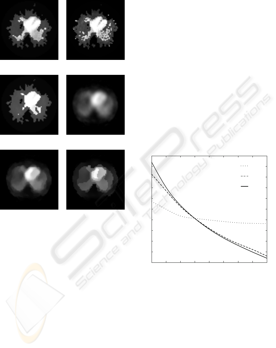
(a) α
1
= 60,α
2
= 10,α
3
= 10 (b) α
1
= α
2
= α
3
= 10
(c) α
1
= α
2
= α
3
= 90 (d) CAR prior
(e) GGMRF prior (f) CGMRF prior
Figure 1: Results with SPECT image.
α
2
, and α
3
were selected experimentally to obtain an
acceptable visual tradeoffbetween detail and noise re-
duction. These parameters were equal to 60, 50, and
32, respectively. Figure 1(a) shows the reconstruction
obtained by the proposed method. The ventricle is
clear in the image and we can observe a small black
area in the left region of the image (possible tumor).
The patient presented a symptomatology compatible
with a hepatic tumor. Small values of α
c
produce very
noisy reconstructions (see Fig. 1(b)), while large val-
ues of α
c
cluster in excess the pixels of the recon-
structed image (see Fig. 1(c), where part of the my-
ocardial wall is not distinguishable).
The variances of the gamma distributions q(x
j
) =
q(x
j
| u
j
,v
j
) provide information about the influence
of the α
c
’s on the reconstruction. These variances
are given by var[x
j
]
q(x
j
|u
j
,v
j
)
= v
2
j
/u
j
. For our experi-
ment, Fig. 2 shows the dependence of the mean of the
above variances on α
1
, α
2
, and α
3
(we plot the curves
that correspond to each α
c
parameter with fixed val-
ues for the other two parameters). We can observe
that the value of α
1
(background and tumor) is not es-
pecially critical for the reconstruction while we need
a more careful selection of the parameters α
2
(liver)
and α
3
(ventricle).
For visual comparison, since the original image is
obviously not available, we show the obtained recon-
struction using several image priors: conditional au-
torregresive (CAR), generalized Gauss Markov ran-
dom fields (GGMRF) and compound Gauss Markov
random field (CGMRF) (see Figs. 1(d), 1(e) and
1(f)), respectively). These reconstructions were ob-
tained with the proposed methods in (L´opez et al.,
2004; L´opez et al., 2002) The area of the tumor is
clearer in the image provided by the reconstruction
using a gamma mixture prior. For example, the lesion
zone does not appear in the obtained reconstruction
with the CGMRF prior (see Fig. 1(f)). We note that in
the proposed method the isotope activity is homoge-
neous in the left ventricle, but it is not homogeneous
in the reconstruction obtained by using the other pri-
ors.
36
37
38
39
40
41
42
43
44
45
46
10 20 30 40 50 60 70 80 90
var
a
1
a
2
a
3
a
Figure 2: Mean of var[x] with respect to α
c
.
6 CONCLUSION
We present a reconstruction method for emission
computed tomography which uses a gamma mixture
as prior distribution to reconstruct Nuclear Medicine
images that present abrupt changes of activity be-
tween contiguous tissues, since spatially independent
priors, as the gamma mixture, are more adapted to this
type of images. We use variational methods to obtain
the original image and parameters estimation within
an unified framework. Satisfactory experimental re-
VARIATIONAL POSTERIOR DISTRIBUTION APPROXIMATION IN BAYESIAN EMISSION TOMOGRAPHY
RECONSTRUCTION USING A GAMMA MIXTURE PRIOR
171

sults are obtained with real clinical images.
ACKNOWLEDGEMENTS
This work has been partially supported by FIS
projects PI04/0857, PI05/1953 and by the Greece-
Spain Integrated Action HG2004-0014.
REFERENCES
Andrieu, C., de Freitras, N., Doucet, A., and Jordan, M.
(2003). An introduction to MCMC for machine learn-
ing. Machine Learning, 50:5–43.
Beal, M. (2003). Variational algorithms for approximate
Bayesian inference. PhD thesis, The Gatsby Compu-
tational Neuroscience Unit, University College Lon-
don.
Bishop, C. and Tipping, M. (2000). Variational relevance
vector machine. In Proceedings of the 16th Confer-
ence on Uncertainty in Articial Intelligence, pages
46–53. Morgan Kaufmann Publishers.
Galatsanos, N. P., Mesarovic, V. Z., Molina, R., and Kat-
saggelos, A. K. (2000). Hierarchical bayesian image
restoration for partially-known blur. IEEE Trans Im-
age Process, 9(10):1784–1797.
Galatsanos, N. P., Mesarovic, V. Z., Molina, R., Katsagge-
los, A. K., and Mateos, J. (2002). Hyperparameter es-
timation in image restoration problems with partially-
known blurs. Optical Eng., 41(8):1845–1854.
Hsiao, I.-T., Rangarajan, A., and Gini, G. (1998). Joint-map
reconstruction/segmentation for transmission tomog-
raphy using mixture-models as priors. In Proceed-
ings of EEE Nuclear Science Symposium and Medical
Imaging Conference, volume II, pages 1689–1693.
Hsiao, I.-T., Rangarajan, A., and Gini, G. (2002). Joint-map
Bayesian tomographic reconstruction with a gamma-
mixture prior. IEEE Trans Image Process, 11:1466–
1477.
Jordan, M. I., Ghahramani, Z., Jaakola, T. S., and Saul,
L. K. (1998). An introduction to variational meth-
ods for graphical models. In Learning in Graphical
Models, pages 105–162. MIT Press.
Kullback, S. (1959). Information Theory and Statistics.
New York, Dover Publications.
Kullback, S. and Leibler, R. A. (1951). On information and
sufficiency. Annals of Mathematical Statistics, 22:79–
86.
Lange, K., Bahn, M., and Little, R. (1987). A theoreti-
cal study of some maximum likelihood algorithms for
emission and transmission tomography. IEEE Trans
Med Imag, 6:106–114.
Likas, A. C. and Galatsanos, N. P. (2004). A variational ap-
proach for Bayesian blind image deconvolution. ieee
j sp, 52(8):2222–2233.
L´opez, A., Molina, R., Katsaggelos, A. K., Rodriguez, A.,
L´opez, J. M., and Llamas, J. M. (2004). Parameter es-
timation in bayesian reconstruction of SPECT images:
An aid in nuclear medicine diagnosis. Int J Imaging
Syst Technol, 14:21–27.
L´opez, A., Molina, R., Mateos, J., and Katsaggelos, A. K.
(2002). SPECT image reconstruction using com-
pound prior models. Int J Pattern Recognit Artif Intell,
16:317–330.
Miskin, J. (2000). Ensemble Learning for Indepen-
dent Component Analysis. PhD thesis, Astrophysics
Group, University of Cambridge.
Miskin, J. W. and MacKay, D. J. C. (2000). Ensemble learn-
ing for blind image separation and deconvolution. In
Girolami, M., editor, Advances in Independent Com-
ponent Analysis. Springer-Verlag.
Mohammad-Djafari, A. (1995). A full bayesian approach
for inverse problems. In in Maximum Entropy and
Bayesian Methods, Kluwer Academic Publishers, K.
Hanson and R.N. Silver eds. (MaxEnt95).
Mohammad-Djafari, A. (1996). Joint estimation of para-
meters and hyperparameters in a bayesian approach
of solving inverse problems. In Proceedings of the
International Conference on Image Processing, pages
473–477.
Molina, R., Katsaggelos, A. K., and Mateos, J. (1999).
Bayesian and regularization methods for hyperpara-
meter estimation in image restoration. IEEE Trans
Image Process, 8(2):231–246.
Molina, R., Mateos, J., and Katsaggelos, A. K. (2006).
Blind deconvolution using a variational approach to
parameter, image, and blur estimation. IEEE Trans
Image Process, 15(12):3715–3727.
Wilks, S. S. (1962). Mathematical Statistics. John Wiley
and Sons.
APPENDIX
In algorithm 3 we need to calculate the quantities
E[x
j
]
q
k
(x)
, E[log(π
c
p
G
(x
j
| β
c
,α
c
))]
q
k+1
(x),q
k+1
(β),q
k
(π)
,
E[1/β
c
]
q
k+1
(β)
and E[logA
i, j
x
j
]
q
k+1
(x)
.
To calculate E[x
j
]
q
k
(x)
we note that (see Eq. 8)
E[x
j
]
p
G
(x
j
|u
j
,v
j
)
= v
j
(61)
To calculate E[1/β
c
]
q
k+1
(β)
we observe with the use of
Eq. 13 that
E
1
β
c
q(β
c
|r
c
,s
c
)
=
=
β
c
((r
c
− 1)s
c
)
r
c
Γ(r
c
)
β
−(r
c
+1)−1
c
e
−(r
c
−1)s
c
/β
c
dβ
c
=
((r
c
−1)s
c
)
r
c
Γ(r
c
)
Γ(r
c
+ 1)
((r
c
−1)s
c
)
r
c
+1
=
r
c
(r
c
−1)s
c
(62)
VISAPP 2007 - International Conference on Computer Vision Theory and Applications
172

We can easily calculate E[logA
i, j
x
j
]
q
k+1
(x)
, since
E[logx
j
]
p
G
(x
j
|u
j
,v
j
)
= −log
u
j
v
j
+
∂logΓ(u)
∂u
|
u=u
j
(63)
where
Γ(u) =
∞
0
τ
u−1
e
−τ
dτ. (64)
(see (Miskin, 2000)). ∂logΓ(u)/∂u is the so called ψ
or digamma function.
To calculate the expectation E[log(π
c
p
G
(x
j
|
β
c
,α
c
))]
q
k+1
(x),q
k+1
(β),q
k
(π)
we note that
E[log(π
c
p
G
(x
j
| β
c
,α
c
))]
q
k+1
(x),q
k+1
(β),q
k
(π)
=
= E[logπ
c
]
q
k
(π)
+ α
c
logα
c
− α
c
E[logβ
c
]
q
k+1
(β)
−logΓ(α
c
) + (α
c
− 1)E[log(x)]
q
k+1
(x)
−α
c
E[
1
β
c
]
q
k+1
(β)
E[x
j
]
q
k+1
(x)
(65)
where E[logπ
c
]
q
k
(π)
can be calculated taking into ac-
count that
E[logπ
c
]
p
D
(π
c
|ω,...,ω
c
)
=
∂logΓ(ω)
∂ω
|
ω=ω
c
−
∂logΓ(ω)
∂ω
|
ω=
∑
C
c
′
=1
ω
c
′
(66)
and E[logβ
c
]
q
k+1
(β
c
)
can be calculated observing that
β
c
follows a distribution p
G
(ρ
c
| m
c
,1/n
c
) and since
E[logβ
c
]
p
IG
(β
c
|m
c
,n
c
)
= −E[logρ
c
]
p
G
(ρ
c
|m
c
,1/n
c
)
(67)
which can be calculated using Eq. 63.
VARIATIONAL POSTERIOR DISTRIBUTION APPROXIMATION IN BAYESIAN EMISSION TOMOGRAPHY
RECONSTRUCTION USING A GAMMA MIXTURE PRIOR
173
