Extraction of Multi–modal Object Representations in a
Robot Vision System
Nicolas Pugeault
1
, Emre Baseski
2
, Dirk Kraft
2
, Florentin W
¨
org
¨
otter
3
and Norbert Kr
¨
uger
2
1
University of Edinburgh
United Kingdom
2
Syddansk Universitet
Denmark
3
G
¨
ottingen University
Germany
Abstract. We introduce one module in a cognitive system that learns the shape
of objects by active exploration. More specifically, we propose a feature tracking
scheme that makes use of the knowledge of a robotic arm motion to: 1) segment
the object currently grasped by the robotic arm from the rest of the visible scene,
and 2) learn a representation of the 3D shape without any prior knowledge of
the object. The 3D representation is generated by stereo–reconstruction of local
multi–modal edge features. The segmentation between features belonging to the
object those describing the rest of the scene is achieved using Bayesian inference.
We then show the shape model extracted by this system from various objects.
1 Introduction
A cognitive robot system should to be able to extract representations about its envi-
ronment by exploration to enrich its internal representations and by this its cognitive
abilities (see, e.g., [10]). The knowledge about the existence of objects and their shapes
is of particular importance in this context. Having a model of an object that includes
3D information allows for the recognition and finding of poses of objects (see, e.g., [8])
as well as grasp planning (e.g. [1], [9]). However, extracting such representations of
objects has shown to be very difficult. Hence many systems are based on CAD models
or other manually achieved information.
In this paper, we introduce a module that extracts multi–modal representations of
objects by making use of the interaction of a grasping system with an early cognitive
vision system (see Fig. 1 and [6]). After gaining physical control over an object (for
example by making use of the object-knowledge independent grasping strategy in [2])
it is possible to formulate predictions about the change of rich feature description under
the object motion induced by the robot.
If the motions of the objects within the scene are known, then the relation between
features in two subsequent frames becomes deterministic (excluding the usual problems
Pugeault N., Baseski E., Kraft D., Wörgötter F. and Krüger N. (2007).
Extraction of Multi–modal Object Representations in a Robot Vision System.
In Robot Vision, pages 126-135
DOI: 10.5220/0002068501260135
Copyright
c
 SciTePress

of occlusion, sampling, etc.). This means that a structure (e.g. in our case a contour) that
is present in one frame is guaranteed to be in the previous and next frames (provided
it does not become occluded or goes out of the field of view of the camera), subject a
transformation that is fully determined by the motion: generally a change of position
and orientation. If we assume that the motions are reasonably small compared to the
frame–rate, then a contour will not appear or disappear unpredictably, but will have a
life–span in the representation, between the moment it entered the field of view and
the moment it leaves it (partial or complete occlusion may occur during some of the
time–steps).
These prediction are relevant in different contexts
– Establishment of objectness: The objectness of a set of features is characterised by
the fact that they all move according to the robot motion. This property is discussed
in the context of a grounded AI planning system in [4].
– Segmentation: The system segments the object by its predicted motion from the
other parts of the scene.
– Disambiguation: Ambiguous features can be characterised (and eliminated) by not
moving according to the predictions.
– Learning of object model: A full 3D model of the object can be extracted by
merging different views created by the motion of the end effector.
In this work, we represent objects as sets of multi–modal visual descriptors called
‘primitives’ covering visual information in terms of geometric 3D information (position
and orientation) as well as appearance information (colour and phase). This represen-
tation is briefly described in section 2. The predictions based on rigid motion are de-
scribed in section 3. The predictions are then used to track primitives over frames and
to accumulate likelihoods for the existence of features (section 4). This is formulated
in a Bayesian framework in section 4.3. In section 5, we finally show results of object
acquisition for different objects and scenes.
2 Introducing Visual Primitives
The primitives we will be using in this work are local, multi–modal edge descriptors that
were introduced in [7] (see figure 1). In contrast to the above mentioned features these
primitives focus on giving a semantically and geometrically meaningful description of
the local image patch. The importance of such a semantic grounding of features for
a general purpose vision front–end, and the relevance of edge–like structures for this
purposes were discussed in [3].
The primitives are extracted sparsely at locations in the image that are the most
likely to contain edges. The sparseness is assured using a classical winner take all op-
eration, insuring that the generative patches of the primitives do not overlap. Each of
the primitive encodes the image information contained by a local image patch. Multi–
modal information is gathered from this image patch, including the position x of the
centre of the patch, the orientation θ of the edge, the phase ω of the signal at this point,
the colour c sampled over the image patch on both sides of the edge, the local optical
127

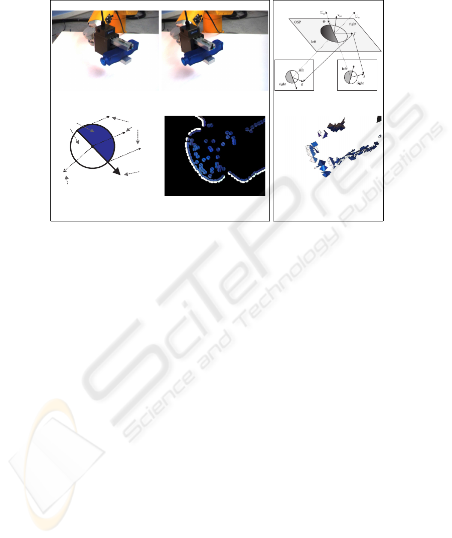
2D 3D
(a) (b) (c)
1)
2)
4)
3)
(d) (e) (f)
Fig. 1. Overview of the system. (a)-(b) images of the scene as viewed by the left and right camera
at the first frame. (d) symbolic representation of a primitive: wherein 1) shows the orientation,
2) the phase, 3) the colour and 4) the optic flow of the primitive. (e) 2D–primitives of a detail
of the object. (c) reconstruction of a 3D–primitive from a stereo–pair of 2D–prim itives. (f) 3D–
primitives reconstructed from the scene.
flow f and the size of the patch ρ. Consequently a local image patch is described by the
following multi–modal vector:
π = (x, θ, ω, c, f , ρ)
T
, (1)
that we will name 2D primitive in the following. The primitive extraction process is
illustrated in Fig. 1.
Note that these primitives are of lower dimensionality than, e.g., SIFT (10 vs. 128)
and therefore suffer of a lesser distinctiveness. Nonetheless, as shown in [11], they
are distinctive enough for a reliable stereo matching if the epipolar geometry of the
cameras is known. Furthermore, their semantic in terms of geometric and appearance
based information allow for a good description of the scene content.
In a stereo scenario 3D primitives can be computed from correspondences of 2D
primitives (see Fig.1)
Π = (X, Θ, Ω, C)
T
, (2)
where X is the position in space, Θ is the 3D orientation, Ω is the phase of the contour
and C is the colour on both sides of the contour. We have a projection relation
P : Π → π (3)
128

linking 3D–primitives and 2D–primitives.
We call scene representation S the set of all 3D–primitives reconstructed from a
stereo–pair of images.
3 Making Predictions from the Robot Motion
If we consider a 3D–primitive Π
t
i
∈ S
t
part of the scene representation at an instant t,
and assuming that we know the motion of the objects between two instants t and t+∆t,
we can predict the position of the primitive in the new coordinate system of the camera
at t + ∆t.
Concretely, we predict the scene representation S
t+∆t
by moving the anterior scene
representation (S
t
) according to the estimated motion between instants t and t + ∆t .
The mapping M
t→t+∆t
associating the any entity in space in the coordinate system of
the stereo set–up at time t to the same entity in the new coordinate at time t + ∆t is
explicitly defined for 3D–primitives:
ˆ
Π
t+∆t
i
= M
t→t+∆t
(Π
t
i
) (4)
Assuming a scene representation S
t
is correct, and that the motion between two
instants t and t + ∆t is known, then the moved representation
ˆ
S
t+∆t
according to
the motion M
t→t+∆t
is a predictor for the scene representation S
t+∆t
that can be
extracted by stereopsis at time t + ∆t.
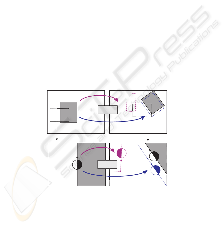
t
t+ td
A
A
A'
t
t+ td
predicted
motion
predicted
motion
p
i
t
p
i
t+ td
p’
A''
P
i k®
P
i j®
p’’
P
i k®
P
i j®
Fig. 2. Example of the accumulation of a primitive (see text).
Note that the predicted representation stems from the primitives extracted from the
cameras at time t whereas the real scene representation is issued from primitives ex-
tracted at time t + ∆t.
129

By extension, this relation also applies to the image representations reprojected onto
each of the stereo image planes I
F
, F ∈ {left,right}, defined by a projection P
F
:
ˆ
π
F,t+∆t
i
= P
F

M
t→t+∆t
(Π
t
i
)

(5)
This prediction/verification process is illustrated in Fig. 2. The left column shows
the image at time t whereas the right column shows the image at time t + ∆t. The top
row shows the complete image of the object and the bottom row shows details of the ob-
ject specified by the black rectangle. If we consider the object A with (solid rectangle in
the top–left and top–right images) that between time t and t + ∆t according to a motion
M
t→t+∆t
Two hypotheses on the 3D shape of the object lead to two distinct predictions
at time t + ∆t: A’ (correct and close to the actual pose of the object, blue rectangle in
the top–right image) and A” (erroneous, red rectangle). In the bottom row, we study the
case of a specific 2D–primitive π
t
i
lying on the contour of A at the instant t (bottom–left
image). If one consider that, at time t, there was two ambiguous stereo correspondences
π
t
j
and π
t
k
then we have two mutually exclusive 3D reconstructions Π
t
i→j
and Π
t
i→k
,
each predicting a different pose at time t + ∆t: 1) the correct hypothesis Π
t
i→j
predicts
a 2D–primitive π
0
that matches with π
t+∆t
i
(blue in the bottom–right image), one of the
a 2D–primitive newly extracted at t+∆t from the contour of A, comforting the original
hypothesis; 2) when moving the incorrect hypothesis Π
t
i→k
we predict a 2D–primitive
π
00
(red in the bottom–right image), that do not match any primitive extracted from the
image, thereby revealing the erroneousness of the hypothesis.
Differences in viewpoint and pixel sampling lead to large variation in the primitives
extracted and the resulting stereopsis. In other words, this means that the same con-
tours of the scene will be described in the image representation, but by slightly shifted
primitives, sampled at different points, along these contours. Therefore we need to de-
vise a tracking algorithm able to recognise similar structures between heterogeneous
representations.
4
If a precise robot like the Staubli RX60 is used to move the objects the motion of
the robot can be used to predict the primitive positions. Hereby it needs to be mentioned
that the primitive position and orientation are usually represented in the camera coor-
dinate system (placed in the left camera) while the robot movements are relative to the
robot coordinate system (for the RX60 this is located at its first joint). To compute the
mapping between the two coordinate systems we use a calibration procedure in which
the robot end effector is moved to the eight positions of a virtual cube. At each location
the position of the end effector in both coordinate systems are noted. The transforma-
tion between the two systems can then be computed by solving the overdetermined
linear equation system represented by the eight positions. We use the RBM estimation
algorithm described in [12] to do this.
4
We note here that the transformation described in this section does not describe the change of
edges for a specific class of occlusions that occurs when round surfaces become rotated. In
these cases the reconstructed edges do not move according to an RBM.
130

4 Tracking 3D-Primitives Over Time
In this section we will address the problem of integrating two heterogeneous scene
representations, one extracted and one predicted that both describe the same scene at the
same instant from the same point of view. The problem is three–fold: 1) comparing the
two representations, 2) including the extracted primitives that were not predicted, and 3)
re–evaluating the confidence in each of the primitives according to their predictability.
4.1 2D Comparison
We propose to compare the two representations in the 2D image plane domain. This
can be done by reprojecting all the 3D–primitives in the predicted representation
ˆ
S
t+∆t
onto both image planes, creating two predicted image representations
ˆ
I
F
t+∆t
= P
F

ˆ
S
t+∆t

, F ∈ {left,right} (6)
Then both predicted image representations
ˆ
I
F
t+∆t
can be compared with the ex-
tracted primitives I
F
t+∆t
. For each predicted primitive
ˆ
π
i
, a small neighbourhood (the
size of the primitive itself) is searched for an extracted primitive π
j
whose position and
orientation are very similar (with a distance less than a threshold t
θ
).
Effectively a given prediction
ˆ
Π
i
is labelled as matched µ(
ˆ
Π
i
) iff. for each image
plane F defined by the projection P
F
and having an associated image representation
I
F
t
, we have the projection π
F
i
= P
x
(Π
i
) satisfy the following relation:
∃π
j
∈ I
F
t
,

d
2D
(
ˆ
π
F
i
, π
j
) < r
2D
,
d
Θ
(
ˆ
π
F
i
, π
j
) < t
Θ
(7)
with r
2D
being the radius of correspondence search in pixels, t
Θ
being the maximal
orientation error allowed for matching, d
2D
stands for the two–dimensional Euclidian
distance, and d
Θ
is the orientation distance. This is also illustrated in Fig. 2.
This 2D–matching approach has the following advantages: First, as we are compar-
ing the primitives in the image plane, we are not affected by the inaccuracies and failures
due to the 3D–reconstruction (see also [5]). Second, using the extracted 2D–primitives
directly allows for 2D–primitives that could not be reconstructed at this time–step due
to errors in stereo matching, etc.
4.2 Integration of Different Scene Representations
Given two scene representations, one extracted S
t
and one predicted
ˆ
A
t
we want to
merge them into an accumulated representation A
t
.
The application of the tracking procedure presented in section 4.1 provides a sep-
aration of the 3D–primitives in S
t
into three groups: confirmed, unconfirmed and not
predicted.
The integration process consist into adding to the accumulated representation A
t−1
,
all 3D–primitives issued from the scene representation S
t
that are not matched by any
3D–primitive in A
t−1
(i. e. the non–predicted ones).
131

A
t
= A
t−1
∪ S
t
(8)
This allows to be sure that the accumulated representation always strictly include
the newly extracted representation (S
t
⊆ A
t
), and enables to include new information
in the representation.
4.3 Confidence Re–evaluation from Tracking
The second mechanism allows to re–evaluate the confidence in the 3D–hypotheses de-
pending on their resilience. This is justified by the continuity assumption, which states
that 1) any given object or contour of the scene should not appear and disappear in and
out of the field of view (FoV) but move gracefully in and out according to the estimated
ego–motion, and 2) that the position and orientation of such a contour at any point in
time is fully defined by the knowledge of its position at a previous point in time and of
the motion of this object between these two instants.
As we exclude from this work the case of independent moving object, and as the
ego–motion is known, all conditions are satisfied and we can trace the position of a
contour extracted at any instant t at any later stage t + ∆t, as well as predict the instant
when it will disappear from the FoV.
We will write the fact that a primitive Π
i
that predicts a primitive
ˆ
Π
t
i
at time t is
matched (as described above) as µ
t
(
ˆ
Π
i
) We define the tracking history of a primitive
Π
i
from its apparition at time 0 until time t as:
µ(Π
i
) =

µ
t
(
ˆ
Π
i
), µ
t−1
(
ˆ
Π
i
), · · · , µ
0
(
ˆ
Π
i
)

T
(9)
thus, applying Bayes formula:
p

Π
i
|µ(
ˆ
Π
i
)

=
p

µ(
ˆ
Π
i
)|Π

p (Π)
p

µ(
ˆ
Π
i
)|Π

p (Π) + p

¯µ(
ˆ
Π
i
)|
¯
Π

p

¯
Π

(10)
where Π and
¯
Π are correct and erroneous primitives, respectively.
Furthermore, if we assume independence between the matches we have, and as-
suming that Π exists since n iterations and has been matched successfully m times, we
have:
p

µ(
ˆ
Π
i
)|Π

=
Q
t
p

µ
t
(
ˆ
Π
i
)|Π

= p

µ
t
(
ˆ
Π
i
) = 1|Π

m
p

µ
t
(
ˆ
Π
i
) = 0|Π

n−m
(11)
In this case the probabilities for µ
t
are equiprobable for all t, and therefore we define
the quantities α = p (Π), β = p

µ
t
(
ˆ
Π) = 1|Π

and γ = p

µ
t
(
ˆ
Π) = 1|
¯
Π

then
we can rewrite (10) as follows:
p

Π
i
|¯µ(
ˆ
Π
i
)

=
β
m
(1 − β)
n−m
α
β
m
(1 − β)
n−m
α + γ
m
(1 − γ)
n−m
(1 − α)
(12)
132

We measured these prior and conditional probabilities using a video sequence with
known motion and depth ground truth obtained via range scanner. We found values of
α = 0.46, β = 0.83 and γ = 0.41. This means that, in these examples, the prior likeli-
hood for a stereo hypothesis to be correct is 46%, the likelihood for a correct hypothesis
to be confirmed is 83% whereas for an erroneous hypothesis it is of 41%. These prob-
abilities show that Bayesian inference can be used to identify correct correspondences
from erroneous ones. To stabilise the process, we will only consider the n first frames
after the appearance of a new 3D–primitive. After n frames, the confidence is fixed
for good. If the confidence is deemed too low at this stage, the primitive is forgotten.
During our experiments n = 5 proved to be a suitable value.
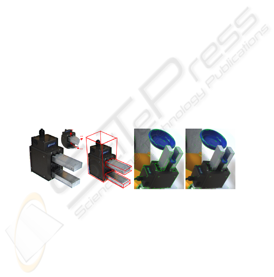
4.4 Eliminating the Grasper
The end-effector of the robot follows the same motion as the object. Therefore, this end-
effector becomes extracted as well. Since we know the geometry of this end-effector
(Figure 3 (a)), we can however easily subtract it by eliminating the 3D primitives that
are inside the bounding boxes that bounds the body of the gripper and its fingers (Fig-
ure 3 (b)). For this operation, three bounding boxes are calculated in grasper coordinate
system (GCS) by using the dimensions of grasper. Since the 3D primitives are in robot
coordinate system (RCS), the transformation from RCS to GCS is applied to each prim-
itive and if the resultant coordinate is inside any of the bounding boxes, the primitive
is eliminated. In Figure 3 (c) 2D projection of 3D primitives extracted from a stereo
pair is presented. After gripper elimination, 2D projection of remaining primitives are
shown in Figure 3 (d).
(a) (b) (c) (d)
Fig. 3. Gripper elim ination (a) grasper and grasper coordinate system (b) bounding boxes of
grasper body and its fingers (c) primitives before grasper elimination (d) primitives after grasper
elimination
5 Results and Conclusion
We applied the accumulation scheme to a variety of scenes where the robot arm manip-
ulated several objects. The motion was a rotation of 5 degrees per frame. The accumu-
lation process on one such object is illustrated in Fig. 4. The top row show the predic-
tions at each frame. The bottom row, shows the 3D–primitives that were accumulated
133

(a) (b) (c) (d)
Fig. 4. Birth of an object (a)-(b) top:2D projection of the accumulated 3D representation and
newly introduced primitives, bottom:accumulated 3D representation. (c) newly introduced and
accumulated primitives in detailed. Note that, the primitives that are not updated are red and the
ones that have low confidence are grey (d) final accumulated 3D representation from two different
poses.
Fig. 5. Objects and their related accumulated representation.
(frames 1, 12, 22, and 32). The object representation becomes fuller over time, whereas
the primitives reconstructed from other parts of the scene are discarded. Figure 5 shows
the accumulated representation for various objects. The hole in the model corresponds
to the part of the object occluded by the gripper. Accumulating the representation over
several distinct grasps of the objects would yield a complete representation.
Conclusion: In this work we presented a novel scheme for extracting object model
from manipulation. The knowledge of the robot’s arm motion gives us two precious
134

information: 1) it enables us to segment the object from the rest of the scene; and 2)
it allows to track object features in a robust manner. In combination with the visually
induced grasping reflex presented in [2], this allows for an exploratory behaviour where
the robot attempts to grasp parts of its environment, examine all successfully grasped
shapes and learns their 3D model and by this becomes an important submodule of the
cognitive system discussed in [4].
Acknowledgements
This paper has been supported by the EU-Project PACOplus (2006-2010).
References
1. C. Borst, M. Fischer, and G. Hirzinger. A fast and robust grasp planner for arbitrary 3D
objects. In IEEE International Conference on Robotics and Automation, pages 1890–1896,
Detroit, Michigan, May 1999.
2. J. Sommerfeld D. Aarno, D. Kragic, N. Pugeault, S. Kalkan, F. W
¨
org
¨
otter, D. Kraft, and
N. Kr
¨
uger. Early reactive grasping with second order 3d feature relations. IEEE Conference
on Robotics and Automation (submitted), 2007. submitted.
3. James H. Elder. Are edges incomplete ? International Journal of Computer Vision, 34:97–
122, 1999.
4. Ch. Geib, K. Mourao, R. Petrick, N. Pugeault, M. Steedman, N. Kr
¨
uger, and F. W
¨
org
¨
otter.
Object action complexes as an interface for planning and robot control. Workshop Toward
Cognitive Humanoid Robots at IEEE-RAS International Conference on Humanoid Robots
(Humanoids 2006), 2006.
5. R.I. Hartley and A. Zisserman. Multiple View Geometry in Computer Vision. Cambridge
University Press, 2000.
6. N. Kr
¨
uger, M. Van Hulle, and F. W
¨
org
¨
otter. Ecovision: Challenges in early-cognitive vision.
International Journal of Computer Vision, submitted.
7. N. Kr
¨
uger, M. Lappe, and F. W
¨
org
¨
otter. Biologically motivated multi-modal processing of
visual primitives. Interdisciplinary Journal of Artificial Intelligence & the Simulation of
Behavious, AISB Journal, 1(5):417–427, 2004.
8. D.G. Lowe. Three–dimensional object recognition from single two images. Artificial Intel-
ligence, 31(3):355–395, 1987.
9. A.T. Miller, S. Knoop, H.I. Christensen, and P.K. Allen. Automatic grasp planning using
shape primitives. In IEEE International Conference on Robotics and Automation, volume 2,
pages 1824–1829, 2003.
10. P. Fitzpatrick and G. Metta. Grounding vision through experimental manipulation. Philo-
sophical Transactions of the Royal Society A: Mathematical, Physical and Engineering Sci-
ences, 361:2165–2185, 2003.
11. N. Pugeault, F. W
¨
org
¨
otter, and N. Kr
¨
uger. Multi-modal scene reconstruction using perc ep-
tual grouping constraints. In Proceedings of the 5th IEEE Computer Society Workshop on
Perceptual Organization in Computer Vision, New York City June 22, 2006 (in conjunction
with IEEE CVPR 2006), 2006.
12. B. Rosenhahn, O. Granert, and G. Sommer. Monocular pose estimation of kinematic chains.
In L. Dorst, C. Doran, and J. Lasenby, editors, Applied Geometric Algebras for Computer
Science and Engineering, pages 373–383. Birkh
¨
auser Verlag, 2001.
135