
A FAST INTERPOLATION METHOD TO REPRESENT THE BRDF
IN GLOBAL ILLUMINATION
Pierre Y. Chatelier
LAIC, Universit
´
e d’Auvergne, Aubi
`
ere, France
R
´
emy Malgouyres
LAIC, Universit
´
e d’Auvergne, Aubi
`
ere, France
Keywords:
Global illumination, BRDF, discrete representation, spherical harmonics, control-points, interpolation, rota-
tion.
Abstract:
Global illumination that simulates realistic lighting environments makes use of bidirectional reflectance dis-
tribution functions (BRDF). Such a function is a surface property, describing how light is re-emitted after
hitting this surface. The present paper details a representation of BRDF and radiance distributions, based
on control points, that aims at performance. It uses spherical triangles for interpolation, least square mean
or linear programming for optimal representation, and very fast rotation by precomputing control points re-
weightening. It has some more advantages for deforming an existing shape. This approach is compared to
Spherical Harmonics, and outperforms this last one.
1 INTRODUCTION
Global illumination that simulates realistic lighting
environments must be able to describe how light is
re-emitted after hitting the surface of an object, de-
pending on the optical properties of this surface: the
material properties. The Lambertian model is one of
the simplest: a fraction of light (depending on the
zenithal incidence) is isotropically re-emitted above
the surface. This is also known as the ideal diffuse
case. In this case, the material property is embedded
in a single factor, as a real number.
However, most objects, like mirrors, velvet, wet
surfaces. . . should not use such a simple model. First,
asymetric materials like velvet must take in account
not only the zenithal angle of an incoming ray, but
also the azimuthal orientation of the ray according to
the surface. Second, incoming light is anisotropically
re-emitted. This is particularly obvious for a perfect
mirror, which is said to be a perfect specular reflec-
tor. Implementing a material mixing up diffuse and
specular properties implies a way to represent spatial
anisotropy.
The notion of Bidirectional Reflectance Distri-
bution Function (BRDF), and radiance distribution,
is the common way to describe such a behaviour.
This paper describes the well known problem of
representing and using BRDFs (Neumann, 2001;
Rusinkiewicz, 1997; Rusinkiewicz, 1998). The re-
quired operations for using them in a global illumi-
nation solver are presented, and we show how they
are addressed with spherical harmonics. Then, we in-
troduce a fast interpolation method, designed to per-
form these operations with maximal performance and
a reasonable precision. Computational experiments
have been performed to compare this method with the
spherical harmonics.
2 USING A BRDF
2.1 Representation
A BRDF function is a function of two parameters:
the direction of incoming light, and the direction of
the outgoing ray for which we want to know the re-
emission. Each direction is in fact a two-dimensional
parameter, usually denoted by the two spherical an-
gles θ and φ, representing elevation and azimuth
(see Fig. 1), so that a BRDF is rather seen as a 4-
dimensional function . The returned value is the ratio,
5
Y. Chatelier P. and Malgouyres R. (2007).
A FAST INTERPOLATION METHOD TO REPRESENT THE BRDF IN GLOBAL ILLUMINATION.
In Proceedings of the Second International Conference on Computer Graphics Theory and Applications - GM/R, pages 5-12
DOI: 10.5220/0002072100050012
Copyright
c
SciTePress

of the reflected (or transmitted) radiance in the given
outgoing direction, to the incoming energy flux from
the incoming direction. The BRDF of an ideal-diffuse
surface is constant, while an ideal reflector can be rep-
resented by a Dirac delta function. A simple BRDF
may be stored as a mathematical function, but arbi-
trary BRDFs usually require a set of sample points
that have to be interpolated. Many representations for
BRDFs have been proposed in the computer graphics
literature (Ward, 1992; Ashikhmin and Shirley, 2000;
Kautz et al., 2002), generally based on a decompo-
sition on a basis of spherical functions, like spher-
ical harmonics or spherical wavelets (Schr
¨
oder and
Sweldens, 1995; Koenderink et al., 1996).
2.2 Models and Instanciations: Brdf
and Radiance Distributions
By stating that we are using a BRDF to modelize light
re-emission, we are only describing how we handle
this material property. However, one must not for-
get that this material property is static and is different
from the effective emission that appears in each ele-
ment that constitutes the surface. Indeed, considering
the 3D scene for which we are computing global illu-
mination, it is usually discretized into several patches,
each patch behaving like a light emitter. Patches from
the same surface will share the same BRDF, that de-
scribes their behaviour. But the effective emission
varies from patch to patch, according to the quantity
of energy that each one is re-emitting, and that has
been computed by the global illumination algorithm.
This effective emission is the radiance distribution,
which is a function of one parameter: the outgoing
direction (see Fig. 2). Here again, it can be seen as a
two-dimensional spherical function on θ and φ. This
function is not known in advance, it is what is com-
puted by the global illumination algorithm. At first,
only the light sources have non-zero radiance distri-
butions. Then, progressively, light propagates and hits
some patches, that affects their radiance distributions
according to their local BRDF. Solving the global il-
lumination problem means that BRDF are known 4-
dimensional functions, while radiance distributions
are the unknowns, 2-dimensional functions.
For the sake of performance, these two kind of
objects are usually represented with the same data
structures. Instead of encoding a 4-dimensional
function, the BRDF can be implemented as the
interpolation of 2-dimensional functions. That is
to say, f (θ
in
, φ
in
, θ
out
, φ
out
) is computed from some
g
θ
in
,φ
in
(θ
out
, φ
out
). Hence, both BRDF and radiance
distributions can be represented by 2D spherical func-
tions, and we only need a way to encode efficiently
θ
out
φ
in
θ
in
φ
out
incoming
outgoing
x
y
z
Figure 1: Polar angles to
define a BRDF. θ is the
zenithal angle (elevation), φ
is the azimuthal angle (ori-
entation).
Figure 2: A radiance dis-
tribution is the response of
a BRDF for some incoming
light. This one has diffuse
and specular behaviour.
such data.
2.3 Operations
As it is stated in Section 2.2, managing radiance dis-
tributions requires to encode 2D spherical functions.
In order to use such data, we must ensure some op-
erations to be easy to perform on the representation.
These operations are querying value, scaling, adding,
and rotating the distributions. Since they are to be
performed very often, they must be very efficient.
2.3.1 Querying Value
The radiance distribution of a scene element evolves
while this element receives light during global-
illumination iterative solving. We must be able to
query at any time the light leaving an element in a
particular direction. This can be done using a mathe-
matical model, which returns a value for some param-
eters. This can also be done with interpolation, which
tries to guess a value according to some neighbor-
hood. The Spherical Harmonics mathematical model
is described in Section 2.4. We propose in Section 3
of this paper an interpolating method.
2.3.2 Scaling and Adding
When some light hits a scene element, its local BRDF
is queried for the matching radiance distribution.
Then this distribution is scaled by the effective incom-
ing energy quantity, and added to the radiance distri-
bution already held by the element. See Figure 3 for
an illustration.
2.3.3 Rotating
Radiance distibutions returned by BRDF queries are
computed in a global system of coordinates. They
have to be rotated to be added to a scene element,
which uses a local system. Indeed, θ is related to the
GRAPP 2007 - International Conference on Computer Graphics Theory and Applications
6

querying
radiance
distribution
the distribution
is scaled
BRDF
scene element
with new radiance
distribution
scene element with
radiance distribution
+ incoming
adding
×
incoming
Figure 3: Scaling and adding radiance distribution.
normal vector of the surface, and the azimuthal angle
is meaningful if the surface has an orientation.
2.4 Common Solution
A common method to fulfill all previous requirements
is to use a decomposition of the radiance distribution
function on a basis of spherical functions. The basis
being known, the radiance distribution is just encoded
by a set of coefficients. Adding and scaling distribu-
tions becomes as easy as adding and scaling the coef-
ficients. Rotation is usually the stumbling block.
2.4.1 Spherical Harmonics
Spherical harmonics are a basis of functions that
suits very well at representing spherical 2D func-
tions (Franc¸ois X. Sillion and Claude Puech, 1994;
Kautz et al., 2002). The spherical harmonics basis is
denoted by Y
l,m
and a function f is decomposed with
C
l,m
coefficients as
f (θ, φ) =
∞
∑
l=0
l
∑
m=−l
C
l,m
Y
l,m
(θ, φ) (1)
The definition of Y
l,m
functions makes use of as-
sociated Legendre Polynomials P
l,m
(x) and a normal-
izing constant N
l,m
(x).
Y
l,m
(θ, φ) =
N
l,m
P
l,m
(cosθ)cos(mφ) if m > 0
N
l,0
P
l,0
(cosθ)
√
2 if m = 0
N
l,m
P
l,−m
(cosθ)sin(−mφ) if m < 0
N
l,m
=
s
2l + 1
2π
(l −|m|)!
(l + |m|)!
P
l,m
(x) =
(1 −2m)
√
1 −x
2
P
m−1,m−1
(x) (l = m)
x(2m + 1)P
m,m
(l = m + 1)
x
2l−1
l−m
P
l−1,m
(x) −
l+m−1
l−m
P
l−2,m
(x) (otherw.)
2.4.2 Cost of the Representation
The representation with spherical harmonics requires
to decide how many coefficients are kept for the de-
composition. Since BRDF are usually rather smooth,
only a few dozens coefficients will be needed. it is
important to keep this number the smallest possible,
because since each scene element will hold a whole
set of coefficients, memory becomes rapidly a criti-
cal resource. A good balance must be found between
the expected precision and the required number of co-
efficients (see Fig. 4). For a real function, only real
coefficients are needed.
Ideal specular reflectors are typical examples of
failure of the assertion about smooth BRDFs. How-
ever, such reflectance should not be handled by a very
high frequency distribution, but algorithmically (Sil-
lion et al., 1991).
(a) (b)
(c)
Figure 4: (a) A spherical shape that is to be approximated.
It is made of a sphere with some stretchings. (b) Spheri-
cal harmonics, 16 coefficients (dotted shape). This is not
enough to approximate the shape. ( c) Spherical harmonics,
64 real coefficients (dotted shape). This is a good approxi-
mation of the spherical shape.
2.4.3 Rotation with Spherical Harmonics
The rotation with spherical harmonics is known to be
the stumbling block of this representation (K
ˇ
riv
´
anek
et al., 2005). It is proved to be a linear opera-
tion (
¨
Ohrstr
¨
om, ; Blanco et al., 1997), by multiply-
ing the vector of coefficients by a particular matrix.
A FAST INTERPOLATION METHOD TO REPRESENT THE BRDF IN GLOBAL ILLUMINATION
7

However, such a matrix may be unpractical in the cir-
cumstances (Erdelyi, 1953).
3 CONTROL-POINTS BASED
BRDF
In order to achieve maximal performance, we propose
a method based on interpolation on spherical trian-
gles. This method requires a reasonable amount of co-
efficients, is precise enough for smooth radiance dis-
tributions, achieves very good performance for com-
mon operations, and suits very well for a direction-
based global illumination solver.
3.1 Interpolation
This simplest way to represent a spherical 2D func-
tion is to sample it on some points. If the polar angles
of these points are fixed, the representation only needs
to store the radius component of the spherical coordi-
nates of these points. Then, two difficulties must be
adressed: choose the set of control points, and choose
an interpolation algorithm.
3.1.1 Choosing the Control Points
The control points must be chosen regularly on the
sphere, so that no region is arbitrarily finer than an-
other. Once dispatched on the sphere, the control
points are radially translated to represent spherical
shapes. A good method to achieve this repartition is to
recursively subdivide a regular polyhedron (Schr
¨
oder
and Sweldens, 1995). For instance, starting from a
icosahedron (12 vertices), one can take the middle of
each edge to divide each face into four new triangles.
The initial polyhedron is an important parameter
for the number of control points you wish to have.
With an icosahedron, the number of points grows
rapidly. At orders 0, 1, 2, 3 of subdivisions, this num-
ber is respectively 12, 42, 162, 642 (Fig. 5 and 6).
As stated in section 2.4.2, each scene element holds
a whole set of coefficients, so that its cardinal should
be kept as small as possible, while being big enough
to allow precise radiance distributions. Our experi-
ments has shown that 162 points are a good compro-
mise (Fig 7). On these pictures, the dots are not the
control points, but some samples interpolated by our
method, using the control points.
3.1.2 Weightening
By subdivising as described above, we can define how
a point is interpolated by the control points.
Figure 5: Icosahedron (or-
der 0 of subdivisions).
Figure 6: Starting with
icosahedron, order 1 of
subdivisions.
(a) (b)
(c)
Figure 7: (a) A spherical shape that is to be approximated.
It is made of a sphere with some stretchings. (b) 42 control
points are used. The result is clearly not precise enough
to approximate the given shape. (c) 162 control points are
used. This is a good approximation of the spherical shape.
Let P be a point to be interpolated. If we project P,
and the control points, on the unit sphere, then the
projection P
0
of P falls into a spherical triangle made
by three of the projected control points on the sphere.
P
0
can also lie on an edge or a vertex in degenerated
cases, but this is not a problem.
Instead of using classical bi-linear interpolation, that
is useful for rasterized triangles in computer graphics,
we can instead weighten the vertices by the ratio of
the triangles areas defined by P
0
and the control points
of the neighborhood. These triangles are spherical tri-
angles and their area is easy to compute with respect
to the formula:
area(ABC) =
b
A +
b
B +
b
C −π (2)
where
b
A,
b
B,
b
C are the angles at the vertices.
Let P be the point to be interpolated, its projection P
0
GRAPP 2007 - International Conference on Computer Graphics Theory and Applications
8

falling into the spherical triangle defined by the pro-
jections C
0
1
, C
0
2
, C
0
3
of the control points C
1
, C
2
and C
3
.
We denote the interpolation by writing
P = ω
1
C
1
+ ω
2
C
2
+ ω
3
C
3
(3)
the unknowns being the weights ω
i
.
These weights can be computed according to the areas
of the spherical triangles formed by the projections.
Let these triangles be denoted by P
0
C
0
1
C
0
2
, P
0
C
0
1
C
0
3
,
P
0
C
0
2
C
0
3
, their areas being respectively α
1
, α
2
, α
3
.
We can set
ω
i
=
α
i
α
1
+ α
2
+ α
3
(4)
to get a normalized weightening system (Figure 8a).
3.1.3 Finding the Triangle
To determine the three control points to be used in
interpolation, we have to quickly compute in which
triangle a point is falling. If we are given the po-
lar angles of this point, it is easy to determine some
possible triangles where it is projected. This only re-
quires the control points to be sorted by parallels and
meridians. Once we have found the two parallels en-
cloising the projected point, we can determine which
neighbour control points on these parallels surround
the projection. Most of the time, more than one tri-
angle are candidate, but some cross products can then
determine easily which is the good one (Figure 8b).
ω
1
=
α
1
α
1
+ α
2
+ α
3
ω
2
=
α
2
α
1
+ α
2
+ α
3
ω
3
=
α
3
α
1
+ α
2
+ α
3
α
3
α
2
α
1
C
1
C
2
C
3
P
(a) (b)
Figure 8: (a) Interpolation on spherical triangles. The
weights w
i
are determined from the areas α
i
. (b) The par-
allel and meridians of the control points help finding candi-
dates holding the projection.
3.2 Representing an Existing Function
We explained in Section 2.2 that even 4D-BRDFs
are modelized using 2D-spherical functions, unify-
ing BRDF and radiance distributions representations.
Therefore, we must provide an efficient way to ap-
proximate a given 2D function, by finding an optimal
set of control points regarding the interpolation algo-
rithm.
To find such an optimal set, we can solve the prob-
lem using Least-Squares Method, or Linear Program-
ming. Let f be the 2D spherical function to inter-
polate, and P
i
(r
i
, θ
i
, φ
i
), i ∈ [0; n] the samples of this
function. Let C
j
(r
j
, θ
j
, φ
j
), i ∈ [0;m] be the control
points (n > m is expected). The unknowns are the r
j
.
Our interpolation method states that P
i
is interpolated
by at most three control points C
1
, C
2
and C
3
. We de-
note that by r
i
= ω
i,1
r
1
+ ω
i,2
r
2
+ ω
i,3
r
3
.
Let X be the unknown vector (r
j
)
j∈[0;m]
of radial co-
efficients of the control points C
j
. Let Y be the vector
(r
i
)
i∈[0;n]
of radial coefficients of the samples P
i
. Let
A be the matrix of the weights of interpolation. Each
line of that matrix is the interpolation of one sample,
and holds at most three non-null weights.
The system to solve is AX = Y . Usually, this system
is over-determined since we get as many samples as
we want, while the number of control points remains
limited. It has likely no solution and only an approxi-
mation is needed.
3.2.1 Least-Squares Method
To solve this system, we can use the Least-Squares
Method and set X = (A
t
A)
−1
Y . This has shown very
good results on smooth functions.
3.2.2 Linear Programming
A common problem of the least-squares method is
that there may be a high local error as long as the er-
ror is low elsewhere. In (Marzais et al., 2006), this
problem is addressed using linear programming. By
minimizing the infinite norm of the error, this method
tries to output results with a locally limited error.
For our problem, that linear programming method
consists in solving Equation 5 to minimize the infi-
nite norm of the error.
−1.h ≤ ((AX −Y )
i
)
i∈[0;n]
≤ 1.h (5)
h is the error that is to be minimized
However, better results are obtained in our case by
minimizing the infinite norm of the relative error
(Equation 6). This causes small scale areas to be less
perturbed, at the cost of less precise big scale areas.
−1.h ≤
(AX −Y)
i
Y
i
i∈[0;n]
≤ 1.h (6)
As a compromise, we obtained best results by divid-
ing with the square root of the value (Equation 7).
−1.h ≤
(AX −Y)
i
√
Y
i
i∈[0;n]
≤ 1.h (7)
Indeed, as it can be seen on Figure 7 (c), some areas
are very well approximated, while other are less pre-
cise. If the maximal error is found around the peaks, it
may be a small error compared to the peak scale, but
a big error compared to the small values of the shape.
A FAST INTERPOLATION METHOD TO REPRESENT THE BRDF IN GLOBAL ILLUMINATION
9

Thus, if the error cannot be less than ε, this may cause
perturbations in the range [−ε;ε]. This would spoil
small scale areas for which ε is not a small value. By
taking the relative error, each area is constrained to be
as good as possible. This is illustrated in Fig. 9, with
a large peak as shape.
(a) (b)
(c)
Figure 9: (a) Linear solving with absolute error may cause
small scale areas to be perturbed. (b) Linear solving with
relative error improves small scale areas but is less precise
on big scale ones. (c) A compromise can be found with
the relative error by dividing by the square root of the value
instead of the value itself.
After many tests, the least-squares method kept
performing a little better than the linear programming
method. Both methods are easy to implement and
may be of interest for complex shapes.
3.3 Deforming Existing Shapes
The set of coefficients characterizing the decompo-
sition of a function, on a basis of functions, cannot
be easily interpreted. Most of the time, the first co-
efficients characterize the shape globally, and addi-
tional coefficients introduce local details; but deform-
ing the shape might have an impact on every coef-
ficient. Therefore, it not easy to deform an existing
shape, just by acting on the coefficients, since the con-
sequences are difficult to foresee.
Our interpolation method has the particularity that
any point is characterized by at most three coefficients
that are very easy to determine. Pulling or pushing a
point away from the center of the shape has an effect
only on these three coefficients. To change the radius
of a point of an existing shape, it is only necessary
to recompute the weights of the three associated con-
trol points. Let us consider P(r, θ, φ) interpolated by
C
1
(r
1
, θ
1
, φ
1
), C
2
(r
2
, θ
2
, φ
2
) and C
3
(r
3
, θ
3
, φ
3
). This is
denoted by r = ω
1
r
1
+ ω
2
r
2
+ ω
3
r
3
Let P
0
(r + δr, θ, φ) be the new point P. Then we must
find δr
1
, δr
2
and δr
3
such that r +δr = ω
1
(r
1
+δr
1
)+
ω
2
(r
2
+ δr
2
) + ω
3
(r
3
+ δr
3
).
A trivial soluion is δr = δr
1
= δr
2
= δr
3
, since
ω
1
(r
1
+ δr) + ω
2
(r
2
+ δr) + ω
3
(r
3
+ δr) =
ω
1
r
1
+ ω
2
r
2
+ ω
3
r
3
| {z }
r
+δr (ω
1
+ ω
2
+ ω
3
)
| {z }
1
However, it is a bad solution since it is just a shift
of the spherical triangle in which P is falling. The risk
is to perturbate other interpolated point too much. A
better approach is to weighten δr
i
by ω
i
, so that a con-
trol point is shifted according to its importance in the
interpolation of P.
For instance, if we require δr
i
to be proportional to
ω
i
r
i
, we just have to divide by
∑
ω
2
j
to normalise.
Hence, the solution we chose is :
δr
i
=
ω
i
∑
j
ω
2
j
δr (8)
3.4 Rotation
To perform an efficient interpolation, our method does
not allow the angles of the control points to change.
Therefore, the rotation cannot be applied to the con-
trol points. It is possible, but too expensive, to recom-
pute the control points by resampling the function,
rotating the samples, and reapplying Least-Squares
Method (or Linear Programming) to get the new con-
trol points. The rotation being a critical function, it
should be more efficient than that.
3.4.1 Permutation Approach
In our control points system, a rotation can be ap-
proximated by a permutation of the control points,
by assigning to each virtually rotated control point,
one (another) of the (non-rotated) control points, most
likely the closest (see Figure 10).
Such a process is very fast since the rotation is then
reduced to a set of pre-computed permutations for rel-
evant angles. The drawback is that the rotation is no
more a continous process, can be transformed into the
Identity for small angles, and that much error can be
accumulated in a sequence of rotations.
To compute the permutation associated to a rota-
tion, a naive method would be to match each virtually
rotated control point to the closest control point, start-
ing from the best matching (with minimal error) and
ending with the worst one. The problem is that it can
GRAPP 2007 - International Conference on Computer Graphics Theory and Applications
10

end with catastrophic matchings since less and less
control points remain free while the matchings occur
(see Figure 11).
To overcome the problem, another strategy can be
adopted: first, the best matching is realized with a
control point C. Then each matching is done the best
possible, starting from the point which is the closest
to C and ending with the furthest one. That prevents a
point to become isolated, with all its neighbours hav-
ing realized a match (monopolizing the control points
around). This would be the cause of a poor matching.
Figure 10: Matching each
virtually rotated control
point (dotted stroke) to the
closest non-rotated point
(plain stroke).
Figure 11: “Best-matchings
first” may end in catas-
trophic matchings if not
enough control points re-
main free. Here, the central
point is poorly matched.
3.4.2 A Continuous Approach
The best representation of the rotated shape would be
found by resampling it, and perform LSM again to
solve the constrained system. It is not affordable, but
makes it obvious that the weights of the control points
should be reconsidered rather than merely permuted.
As a matter of fact, it is rather easy to perform, by in-
terpolating the virtually rotated control points on the
original, non-rotated, control points.
Each control point, when rotated, can be seen as a
sample, that is to be interpolated by three “real” con-
trol points. Thus, a “real” control point can be in-
volved in the interpolation of many “virtually rotated”
control points. It is given one weight per interpola-
tion. Then, its new radial distance is set according to
a weighted sum of the interpolations for which it is
participating. Its new position is a compromise and
does not necessarly satisfy each interpolation, but this
simplified processus gives us a simple, continuous ro-
tation method.
3.5 Direction-Driven Global
Illumination Solver
Global illumination algorithms usually use patches as
scene elements, and gathers for each patch the quan-
tity of light received by other patches visible from
there. By iterating this algorithm, light propagates in
the scene and converges towards a radiosity solution.
Another approach presented in (Chatelier and Malgo-
uyres, 2006) uses a special method to compute visi-
bility between volumetric scene elements, and the ra-
diosity algorithm is then parametrized by a set of di-
rections in space to consider. Light is transported only
on these directions. This comes from the fact that vis-
ibility computations are factorized along some rays
(Figure 12).
A consequence of this direction-driven radiosity
solver is that it is also possible to factorize computa-
tions that are done along a ray. Indeed, the interpola-
tion method described in the present paper computes
weights for a given direction (θ, φ). Combined with
the direction-driven solver, this computation can be
factorized for all the scene elements that lie along a
ray. It results in an additional optimization that our
method brings to global illumination solving.
This is not a marginal optimization. We have also
used our BRDF representation in the radiative trans-
fer problem (Lenoble, 1993); in this problem, a cloud
is illuminated and the energy propagations occur ac-
cording to some distributions that are called phase
functions. These phase functions can be represented
by 2D spherical functions. Only one global coordi-
nate system is used, since the volumic elements that
are representing the cloud are not oriented. So, no
rotation is needed. In this context, if N voxels are en-
coding the cloud, each one is queried for its radiance
distribution in the current direction (θ, φ). Then, the
computation of the weights for (θ, φ) can be factor-
ized for the N voxels.
Figure 12: A direction-driven algorithm can factorize the
weights computation of all elements lying along a ray, when
querying values from radiance distributions.
4 EXPERIMENTAL RESULTS
To compare our implementation of BRDFs using
control points, with an implementation using Spher-
ical Harmonics, we have used our radiosity solver
(Chatelier and Malgouyres, 2006). The spherical
harmonics relies on the SpharmonicKit (Kostele and
Rockmore, 2004), which performs very well, so that
the performance gap should not be a defect of our
implementation of the spherical harmonics.
Figure 13 shows that our method largely outperforms
the spherical harmonics approach. Moreover, we
did not implement the rotation of the spherical
A FAST INTERPOLATION METHOD TO REPRESENT THE BRDF IN GLOBAL ILLUMINATION
11
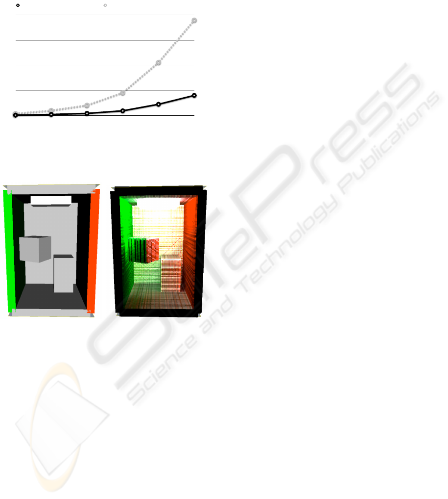
harmonics, so that it is not even slowed down by
their known bottleneck. The scene that has been used
is a very simple assemblage of cubes, with diffuse
BRDFs. It has been discretized into 13000 voxels for
the solver.
45 111 223 489 1131 2013
19
45
89
195
451
808
4
10
19
41
96
171
Control Points (162 coeffs) Spherical Harmonics (64 coeffs)
13000 voxels, 5 itérations
number of directions
seconds
Figure 13: The performance of the control points method
(plain stroke) is far better than the spherical harmonics.
(a) (b)
Figure 14: (a) Simple scene. (b) Raw data per voxel after
radiosity solving.
REFERENCES
Ashikhmin, M. and Shirley, P. (2000). An anisotropic
Phong BRDF model. Journal of Graphics Tools: JGT,
5(2):25–32.
Blanco, M. A., Florez, M., and Bermejo, M. (1997). Evalu-
ation of the rotation matrices in the basis of real spher-
ical harmonics. J. Molecular Structure (Theochem),
419:19–27.
Chatelier, P. Y. and Malgouyres, R. (2006). A low-
complexity discrete radiosity method. Computers &
Graphics, 30:37–45.
Erdelyi, A. (1953). Higher transcendental functions, vol-
ume 2. McGrawHill book company, Inc.
Franc¸ois X. Sillion and Claude Puech (1994). Radiosity &
Global Illumination. Morgan Kaufmann Publishers,
Inc.
Kautz, J., Sloan, P.-P., and Snyder, J. (2002). Fast, arbi-
trary brdf shading for low-frequency lighting using
spherical harmonics. In EGRW ’02: Proceedings of
the 13th Eurographics workshop on Rendering, pages
291–296.
Koenderink, J. J., van Doorn, A. J., and Stavridi, M.
(1996). Bidirectional reflection distribution function
expressed in terms of surface scattering modes. In
ECCV ’96: Proceedings of the 4th European Con-
ference on Computer Vision-Volume II, pages 28–39,
London, UK. Springer-Verlag.
Kostele, P. and Rockmore, D. (2004). The
SpharmonicKit and S2Kit libraries.
http://www.cs.dartmouth.edu/ geelong/sphere.
K
ˇ
riv
´
anek, J., Konttinen, J., Bouatouch, K., Pattanaik, S.,
and
ˇ
Z
´
ara, J. (2005). Fast approximation to spherical
harmonic rotation. In SCCG ’06: Proceedings of the
22nd spring conference on Computer graphics (to ap-
pear), New York, NY, USA. ACM Press.
Lenoble, J. (1993). Atmospheric Radiative Transfer. A.
Deepak Publishing.
Marzais, T., Grard, Y., and Malgouyres, R. (2006).
l p−fitting approach for reconstructing parametric sur-
faces from point clouds. In International Confer-
ence on Computer Graphics Theory and Applications,
Set
´
ubal, Portugal, pages 325–330.
Neumann, A. (2001). Constructions of Bidirectional Re-
flection Distribution Functions. PhD thesis, Institute
of Computer Graphics and Algorithms, Vienna Uni-
versity of Technology, Favoritenstrasse 9-11/186, A-
1040 Vienna, Austria.
¨
Ohrstr
¨
om, M. Spherical harmonics, precomputed radiance
transfer and realtime radiosity in computer games.
http://citeseer.ist.psu.edu/685526.html.
Rusinkiewicz, S. (1997). A survey of brdf
representation for computer graphics.
http://www.cs.princeton.edu/˜smr/cs348c-
97/surveypaper.html.
Rusinkiewicz, S. (1998). A new change of variables for effi-
cient BRDF representation. In Drettakis, G. and Max,
N., editors, Rendering Techniques ’98 (Proceedings of
Eurographics Rendering Workshop ’98), pages 11–22,
New York, NY. Springer Wien.
Schr
¨
oder, P. and Sweldens, W. (1995). Spherical wavelets:
efficiently representing functions on the sphere. Com-
puter Graphics, 29(Annual Conference Series):161–
172.
Sillion, F. X., Arvo, J. R., Westin, S. H., and Greenberg,
D. P. (1991). A global illumination solution for gen-
eral reflectance distributions. In SIGGRAPH ’91: Pro-
ceedings of the 18th annual conference on Computer
graphics and interactive techniques, pages 187–196,
New York, NY, USA. ACM Press.
Ward, G. J. (1992). Measuring and modeling anisotropic re-
flection. In SIGGRAPH ’92: Proceedings of the 19th
annual conference on Computer graphics and interac-
tive techniques, pages 265–272, New York, NY, USA.
ACM Press.
GRAPP 2007 - International Conference on Computer Graphics Theory and Applications
12
