PLAUSIBLE MOTION SIMULATION: INCHWORM VS. ROLLER

Juha Holopainen

Department of Computer Science, University of Kuopio

PO Box 1627, 70211 Kuopio, Finland

Mauno R

onkk

Department of Computer Science, University of Kuopio

PO Box 1627, 70211 Kuopio, Finland

Keywords:

Particle systems, plausible motion simulation, intelligent control, emergent dynamics.

Abstract:

In this paper, we study the use of a speciﬁc particle system in motion simulation. The novelty of the particle

system is that, with it, everything is formalized in a systematic and uniform manner using just six matrices.

We illustrate use of the particle system by presenting a challenging environment where two different entities,

Inchworm and Roller, are tested and their behavior is examined. As the main contribution, we demonstrate

here that, despite its simplicity, the particle system supports plausible motion simulation for organic and mech-

anistic motion. In addition, as the entities are modeled in a systematic and uniform manner, they are reusable.

1 INTRODUCTION

Objects and substances displaying emergent dynam-

ics are often simulated with particle systems (Eber-

hardt et al., 1996; Wejchert and Haumann, 1991;

Witkin, 1997; Wojtan et al., 2006).

Here, we present a particle system (R

onkk

2006b) which captures a wide range of dynamics

without being too complex. This is achieved by for-

malizing the components in a systematic and uniform

manner using matrices, as discussed in Section 2.

Due to the formalization, the particle system is

modular, and the components can be reused in dif-

ferent settings. Furthermore, because the interaction

of the components arises as emergent dynamics, the

components automatically adapt to the new settings.

As the main contribution, we demonstrate here

with two active entities that the particle system sup-

ports plausible motion simulation for both organic

and mechanistic motion.

The two entities are Inchworm and Roller, which

are introduced in Sections 3 and 4 respectively. Inch-

worm is an organic entity displaying life-like motion.

Roller, in turn, is a mechanical entity, displaying clas-

sical mechanics. The entities were tested on different

terrains. The terrain which revealed the most interest-

ing dynamics, along with the test runs, is presented in

Section 5. The implications and the plan for further

development are then discussed in Section 6.

2 THE PARTICLE SYSTEM

In the particle system (R

onkk

o, 2006b), there is a

ﬁxed and ﬁnite number of particles. They are unit

balls with uniformly distributed, constant unit mass.

The particles are modeled using six matrices. The

matrices p, v, d, and m capture the position, velocity,

damping coefﬁcient, and memory, respectively. The

matrices b and c indicate which particles are bound

to each other or collide with each other. The particles

are identiﬁed by the rows of the matrices. The values

of p

, v

, and m

are three-dimensional vectors, and

is a real valued number. Lastly, b and c are square

matrices, where any b

and c

is either 0 or 1.

The dynamics of all the particles are governed by

a model of motion. It is a numerical approximation

of the trivial model of motion with forward error cor-

rection. Let t denote a ﬁxed time step, B denote a

bond function, C denote a collision function, R de-

note a model speciﬁc reaction function, and M denote

a model speciﬁc memory update function. Then, the

motion of a particle i is computed:

= p

+ tv

= d

+ B

(p) + C

(p) + R

(p, v, m)

= M

(p, m)

Here, the updated position, p

, is computed using

the updated velocity, v

, which is computed using af-

Holopainen J. and Rönkkö M. (2007).

PLAUSIBLE MOTION SIMULATION: INCHWORM VS. ROLLER.

In Proceedings of the Second International Conference on Computer Graphics Theory and Applications - AS/IE, pages 71-74

DOI: 10.5220/0002073500710074

 SciTePress

fecting forces. The binding forces are computed with

respect to the initial positions, denoted by p

, as:

(p) =

− p

)(1 −

− p

)

Similarly, the collision forces are computed as:

(p) =

− p

) min{0, 1 −

− p

}

In short, the binding forces try to maintain the initial

distance between the particles designated by b. The

collision forces push apart any overlapping particles

that are allowed to collide by c. Two particles overlap,

when their distance is less than the sum of their radii.

When modeling, we ﬁrst assign particles to the

components. We then deﬁne the initial values for p,

m, d, b, and c. The matrix v is zero initially. Lastly,

we deﬁne the functions R and M . The simulation is

then an iterative computation of the model of motion.

In the following, we assume t = 0.01 as the time

step. Also, we use a conditional expression hP i,

which returns 1 if the predicate P holds and 0 oth-

erwise.

3 INCHWORM

Inchworm, presented originally in (R

onkk

o, 2006b),

is similar to Arctic Caterpillar (Miller, 1988). It has

a body and two leg particles. The body is composed

of 60 particles, forming a muscle that operates in two

phases: it contracts and relaxes, as captured in Figure

1. When contracting Inchworm grasps on to the road

with its front leg, and when relaxing, it grasps on to

the road with its tail leg. Contraction and relaxation

are repeated sequentially, lasting the same number of

iteration rounds. For this purpose, Inchworm uses a

memory. In the sequel, we identify a particle i with:

b ody(i) = h0 ≤ i < 60i

legs(i) = h60 ≤ i < 62i

road(i) = h62 ≤ ii

Consider a body particle i of Inchworm, that is

body(i) = 1, and any particle j. Then, the model of

the body is:

= (15, 4, −0.3i + 5)

= (0, 0, 0)

= 0.95

= (1 − road(j)) · h0 < kp

− p

k < 2.5i

= road(j) + (1 − road(j))h2.5 < kp

− p

(p, v, m) = 0.1h0 < m

(i,1)

ih15 ≤ i < 45i · (p

− p

)

(p, m) = (m

(i,1)

+ 1, 0, 0) − (2000h999 < m

(i,1)

i, 0, 0)

Consider a leg particle i and any particle j. Also, let

α be the nearest road particle, so that the condition

road(α) ∧min

2000

k=62

{kp

−p

k} = kp

−p

k holds.

Let β indicate when the leg particle i is supposed to

Figure 1: Inchworm edging its way; the state after the ﬁrst

contraction on the left, and the state after the ﬁrst relaxation

on the right.

Figure 2: Roller from the side and from the top. In the

left image, the left side beam misses the road. In the right

image, the right side beam misses the road.

move, that is, β = hi = 60ihm

(0,1)

< 0i+ hi = 61ih0 ≤

(0,1)

i Lastly, let γ be the value 1 − β. Then, the

model of the legs is:

= (15.3, 3.8, −15.3(i − 60) + 4.1)

= p

= 0.95

= body(j) · h0 < kp

− p

k < 2.5i

= road(j)

(p, v, m) = 0.5(p

− p

)

+ 0.2βhi = 60i(p

− p

) + γ(m

− p

)

(p, m) = γm

+ βp

4 ROLLER

Roller is a system composed of an axle and two

wheels. A simpler version of Roller was presented

earlier in (Holopainen and R

onkk

o, 2006).

The control technique comprises of an observa-

tion technique and a steering technique. The observa-

tion technique uses four beams, as shown in Figure 2,

to detect if there are road particles ahead. Two front

beams observe the ground directly at the front of the

wheels. Two side beams observe the ground slightly

outwards from the front beams.

Based on the observations, the steering technique

steers Roller by rotating one or both of the wheels.

When both of the wheels rotate to the same direction,

Roller moves to that direction. If only one wheel ro-

tates, Roller turns. Roller never rotates wheels to op-

posite directions, as it results in less controllable mo-

tion.

Roller has ﬁve steering decisions, shown in Table

1. The decision is based on the beam status. In the

table, the numbers show if the wheels are rotated for-

wards (1), backwards (-1), or freely (0).

GRAPP 2007 - International Conference on Computer Graphics Theory and Applications

Table 1: Decision table for goal directions.

Beams missing the road Goal direction

none ω

= 1 ω

= 1

only left side beam ω

= 0 ω

= −1

only right side beam ω

= −1 ω

= 0

both left and right side beams ω

= −1 ω

= −1

left or right front beam ω

= −1 ω

= −1

For identifying the component of Roller’s particle

i, we use the functions:

wheel(i) = h0 ≤ i < 40i

axle(i) = h40 ≤ i < 79i

road(i) = h79 ≤ ii

As Roller does not use memory, the model for an

axle particle i, with respect to any other particle j, is:

= ((i − 40)/3 − 7, 6, 1.5)

= 0.999

= (1 − road(j))hi 6= ji

= road(j)

(p, v, m) = (0, −0.32, 0)

Consider a wheel particle i and any particle j.

Also, for i, let α = i div 20, β = j div 20, and

γ = i mod 20. Then, the model is:

= 2.1(5α, cos(0.2πγ), sin(0.2πγ)) + (−6, 6, 1.5)

= 0.999

= wheel(j)hα = βihi 6= ji + axle(j)

= road(j)

As mentioned earlier, the observation technique

uses four beams. Formally, all the beams are identi-

ﬁed by an origin, ~o, and a directional vector, ~r. Let

norm(v) denote the normalized vector of v, that is

norm(v) =

kv k

. Let ~a be an axle vector, that is,

~a = p

− p

, and let ~y be ~y = (0, 20, 0). Then,

the axle’s normal is ~n = norm(~a × ~y), and a planar

normal is ˜n = (3~n

, ~n

, 3 ~n

). Now, the four beams

are deﬁned using cross products:

left front beam: ~o = p

~r = (9~n

, 20, 9 ~n

) × ~a

left side beam: ~o = p

~r = (7~n

, 20, 7 ~n

) × (~a + ˜n)

right front beam: ~o = p

~r = (9~n

, 20, 9 ~n

) × ~a

right side beam: ~o = p

~r = (7~n

, 20, 7 ~n

) × (~a − ˜n)

Consider a beam ~r originating from ~o, and a vector

~p capturing the difference from ~o to a (road) particle

i, that is, ~p = p

−~o. Then, the beam hits the particle

i, if k~p − (

~p•~r

k~rk

)

k~rk

k <

√

1.5 holds.

The steering technique is captured by the reaction

function for the wheel particles. The reaction func-

tions are actually composed of three forces: gravity,

friction, and steering forces. Formally, the reaction

function for the left wheel particle i is stated using a

control force variable θ

as the sum of the three forces:

(p, v, m)

= (0, −0.32, 0)

− 0.02h∃k > 79 : kp

− p

k < 2iv

+ θ

norm((p

− p

) × (p

− p

))

Here, θ

captures a bounded control force with re-

spect to a desired momentum φ

= max(−10, min(φ

, 10))

The desired momentum, φ

, is computed with re-

spect to the goal direction, ω

, and the current direc-

tion, ς, of the left wheel based on the current momen-

tum as:

= −20ω

+ hω

6= 0i

k=0

− v

The goal direction, ω

, is obtained from Table 1.

The current direction, in turn, is computed by com-

paring the velocities of the wheel particles headed for-

ward, σ(k), to all of the wheel particles:

ς =



k=0

(2σ(k) − 1)v

(i,2)

< 0

−1, else

Here, the function σ(k) is computed with re-

spect to the topmost wheel particle, τ , for which

max

k=0

(k,2)

) = p

(τ,2)

, and to the lowest wheel

particle, β, for which min

k=0

(k,2)

) = p

(β,2)

, as:

σ(k) = (hτ > β ∧ k > τi + hτ > β ∧ k < βi)

· hτ < β ∧ τ < k ∧ k < βi

The steering for the right wheel is analogous to the

steering of the left wheel presented above.

5 MOTION ON ROUGH ROAD

We study the motion of Inchworm and Roller on

Rough Road. Rough Road is a narrow uneven path,

having also variation in altitude. Rough Road con-

sists of 1800 immobile particles. Thus, the shape is

exhaustively captured by the initial positions. Techni-

cally, Rough Road consists of 60 circles, each having

30 particles, as observable in Figure 3. For Rough

Road, we identify the a road particle i with road(i) =

h100 ≤ i < 1900i. Let i be a road particle, that

is road(i) = 1. Also, let α = (i − 100) div 30,

β = (i − 100) mod 30, and γ =

π. Then, the ini-

tial positions are captured:

= (8, 0.5(α mod 2), 8)

+hα > 30i(0,

α, 0) + hα ≤ 30i(0, (11 −

α), 0)

+30(cos(0.5αγ), 0, sin(αγ)) + 8(cos(2βγ), 0, sin(2βγ))

PLAUSIBLE MOTION SIMULATION: INCHWORM VS. ROLLER

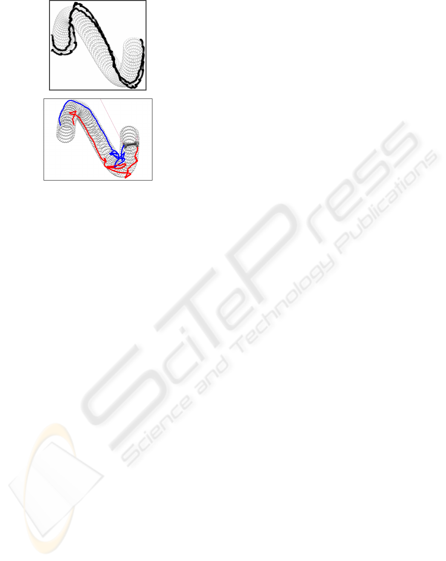
Figure 3: Inchworm (top) and Roller (bottom) on Rough

Road. Travelling direction is from left to right.

As the easiest road for both entities is a ﬂat straight

road, Rough Road offers many challenges; the shape

varies in all dimensions and the surface is bumpy.

The motion of Inchworm is orientation indepen-

dent, and it makes no predictions of the road ahead. It

has a tendency to go straight forward and follow the

edges of the road.

Road altitude variations are problematic for

Roller. As the observation beams are directed to a

constant downward angle, Roller has tendency to un-

dersteer and oversteer in downhills and uphills. Roller

tries to make predictions of the road ahead and keep

both wheels in a safe distance from the edges. In this

respect, Rough Road is wide enough. Roller is suc-

cessful in the ﬁrst curve, and the problems in the sec-

ond curve are the result of the rough surface.

Contrary to Inchworm that grips tightly to the road

surface and slides slowly along the surface, only the

undermost wheel particles of Roller touch the road.

Therefore, Roller has problems with bumpy road sur-

face especially in the inner corner of the second curve,

where the road elevates sharply.

Figure 3 shows that Roller has a more mechanis-

tic motion than Inchworm. Also, Roller ﬁnds its way

forward by trial and error, whereas Inchworm edges

forward smoothly but stubbornly.

6 DISCUSSION

In this paper we studied the use of a speciﬁc particle

system in motion simulation. The novelty of the par-

ticle system is that, with it, everything is formalized

systematically and uniformly with matrices.

The results of this study were twofold: First, we

demonstrated the applicability of the particle system

in simulating plausible motion dynamics. Secondly,

we examined the reusability of components that were

formalized using the particle system. In this paper, we

demonstrated the behavior of Inchworm and Roller.

They displayed very different motion dynamics.

The results of this paper complement our ear-

lier results (Holopainen and R

onkk

o, 2006; R

onkk

2006b). In particular, the reusability results encour-

age us to ﬁnd out what kind of interactive tools and

techniques could be used for shaping and formalizing

particle system components.

We used Atoms (R

onkk

o, 2006a) for computing

the simulations in this paper. Currently, Atoms is not

adequate for running large models. Thus, an impor-

tant topic for future research is to ﬁnd out how to im-

prove the performance of Atoms.

ACKNOWLEDGEMENTS

We wish to thank Vivian Michael Paganuzzi, as well

as members of Garry Wong’s laboratory.

REFERENCES

Eberhardt, B., Weber, A., and Strasser, W. (1996). A

fast, ﬂexible, particle-system model for cloth draping.

Computer Graphics and Applications, 16(5):52–59.

Holopainen, J. and R

onkk

o, M. (2006). Embedding control

into a particle system: a case study. In Proceedings of

the Ninth IASTED International Conference on Intel-

ligent Systems and Control, pages 92–97. Acta Press,

Anaheim.

Miller, G. (1988). Motion dynamics of snakes and worms.

Computer Graphics, 22:169–178.

onkk

o, M. (2006a). Atoms: software development kit.

Department of Computer Science, University of Kuo-

pio. http://www.cs.uku.ﬁ/research/GPL/atoms.tar.

onkk

o, M. (2006b). Hybrid systems: Modeling and anal-

ysis using emergent dynamics. Accepted to Nonlinear

Analysis: Theory, Methods & Application s.

Wejchert, J. and Haumann, D. (1991). Animation aero-

dynamics. In Proceedings of the 18th Annual Con-

ference on Computer Graphics and Interactive Tech-

niques, pages 19–22. ACM Press, New York.

Witkin, A. (1997). Physically Based Modeling: Principles

and Practice. Online Siggraph ’97 Course notes.

Wojtan, C., Mucha, P., and Turk, G. (2006). Keyframe

control of complex particle systems using the ad-

joint method. In Proceedings of ACM SIG-

GRAPH/Eurographics Symposium on Computer An-

imation, pages 15–23.

GRAPP 2007 - International Conference on Computer Graphics Theory and Applications