
TILING THE SPHERE WITH DIAMONDS
FOR TEXTURE MAPPING
John E. Crider
32919 Leafy Oak Court, Magnolia TX 77354-6566 USA
Keywords: Coordinate system, mapping, quadrilateral, sphere, texture, tiling.
Abstract: The sphere can be covered by any of an infinite number of tiling sets of equilateral spherical quadrilaterals
(diamonds). Five of these tiling sets have practical use for texture mapping application. Points on the sphere
can be described by intersections of geodesics, which provide coordinate values in a new coordinate system,
defined for each tiling set. Each of the diamonds can be subdivided by a grid of coordinate geodesics to
pixel level and so can be directly mapped to and from a texture array. The diamonds can also be subdivided
into spherical quadrilaterals that can be approximated by pairs of triangles for fast rendering in a graphics
system. Because coordinates in the new system are readily converted to and from Cartesian coordinates,
diamonds can be used easily in interactive graphics and ray-tracing applications.
1 INTRODUCTION
Texture mapping is essentially the mapping of an
image onto the surface of a graphics object. The
image is typically a square array of discrete elements
called texels. In this paper, a texel is also the
quadrilateral on the surface of the sphere that
corresponds to an element in the texture array.
The image also has its own coordinate space,
usually with coordinates denoted as (u, v). The
coordinates typically run from 0 to 1; in this way,
the number of elements in the array (i.e., the
resolution) can be changed without affecting the
mapping mathematics.
A necessary part of texture mapping is the
mapping function, through which a point on the
surface of the object (expressed perhaps in Cartesian
coordinates in object space or in a surface coordinate
system) is mapped to a point in the coordinate space
of the texture image (Foley, van Dam, Feiner, and
Hughes, 1996; Heckbert, 1986).
Watt and Watt (1982) discuss texture mapping in
general and texturing the sphere specifically. The
discussed technique divides the surface of the sphere
into areas that are delimited by circles of constant
latitude and longitude. However, such areas do not
lead to a consistent set of tiles; in particular, polar
areas usually require special treatment.
One common approach to texturing a sphere is to
use a texture array in which the rows correspond to
latitude and the columns correspond to longitude.
This single-tile approach has several disadvantages.
The texels at the poles are extremely small in area, a
waste of texture resources. Further, a graphics
engine that limits the size of texture arrays would
prevent the increase in size of the texture array to
achieve high resolution.
Texturing a sphere through a set of tiles provides
several advantages. First, because each tile covers a
relatively small portion of the spherical surface, it
can have low area distortion and thus can make
economic use of texture resources. Second, a set of
tiles, with a separate texture array mapped to each
tile, can obviously provide higher resolution than
can a single texture array mapped to the whole
sphere. This advantage is especially important with
graphics engines that have restraints on sizes of
texture arrays affecting performance.
The goal here is to cover the sphere with tiles of
identical size and shape such that a texture array can
be easily mapped to each tile. High resolution is
another desirable goal.
The literature on spherical tilings does not
address texture mapping, and the various schemes
described are intended for other applications and are
not usually well suited to texture mapping.
For example, Borgefors (1992) describes a
spherical tiling in which the application is a view-
sphere for image analysis. Each hemisphere is
divided into four tiles of equal area; each tile is then
116
E. Crider J. (2007).
TILING THE SPHERE WITH DIAMONDS FOR TEXTURE MAPPING.
In Proceedings of the Second International Conference on Computer Graphics Theory and Applications - GM/R, pages 116-123
DOI: 10.5220/0002074701160123
Copyright
c
SciTePress

recursively divided into four. Each level includes
polar tiles with circular borders, figures that are
difficult to map to texture arrays. At any subdivision
level, the tiles are equal in area but quite different in
shape.
One well-known approach to tiling the sphere is
to begin with the tiling set of twenty equilateral
spherical triangles based on the vertices of an
inscribed regular icosahedron. Finer triangulations
are then obtained by recursively subdividing the
spherical triangles into four with geodesics (Pottman
and Eck, 1990; Ramaraj, 1986). An inscribed
tetrahedron has also been used (Nielson, 1993;
Renka, 1984). The common application for these
tilings is data interpolation.
A similar approach of recursive triangulation is
based on an inscribed regular octahedron (Dutton,
1999); the application is GIS. The hierarchical
coordinate system described is a quad-tree encoding,
not a traditional coordinate system with continuous
coordinates. The recursive subdivisions are based on
latitude and longitude, not geodesics. Other GIS-
related tilings include an equal-area hierarchical
tiling (Wickman, Elvers, and Edvarson, 1974) based
upon a dodecahedron and a tiling (White, Kimerling,
and Overton, 1992) based upon a truncated
icosahedron, or “soccer ball.”
However, when applied to texture mapping, a
recursive triangulation approach has two problems.
First, when the triangular tiles are subdivided to
texel level, the texel figures are triangular and in a
triangular pattern, and are difficult to match with
elements in a square texture array. Conceptually,
there appears to be a simple solution: adjacent
triangular icosahedral tiles can be paired to form a
tiling set of ten quadrilaterals, and the texel triangles
can be similarly paired, forming a matchable pattern
of quadrilateral texels in a quadrilateral grid.
However, in application, recursive triangulation is
essentially the traversal of a quad-tree structure, and
adjacent texel triangles to be paired may be widely
separated in the tree, which can lead to a
complicated scheme for associating these triangles.
Borgefors (1992) states that the recursive
triangulation from icosahedral vertices does not
provide an easy way to determine in which sub-tile
an arbitrary point is located. (This determination is a
complicated recursive calculation involving
numerous geodesics.) Thus, the second problem is
that recursive triangulation lacks a convenient
mapping of arbitrary points from object space to
texture image space; it is not suitable for texture
mapping.
Another approach (Giraldo, 2001) from
icosahedral spherical triangles is to connect the
center of each triangle with the center of each of the
edges, thus forming three spherical quadrilaterals.
The quadrilaterals have two opposite angles of 90°;
the other two angles are 120° and 72°. The
application is fluid dynamics modelling. The
described mapping is through the gnomonic map
projection.
Górski et al. (2005) describe several quadrilateral
tilings derived from the cylindrical equal-area map
projection; sub-tilings are also equal-area. However,
the quadrilaterals in a tiling set are not of the same
shape. Also, polar quadrilaterals require separate
treatment. Designed for processing astronomical
data, this approach reduces the number of latitudes
on which pixels are centered, a concern that is not
relevant for texturing.
One useful technique for texturing the sphere
through tiling is based on Fuller’s map projection
(Gray, 1995). This patented (Fuller, 1946) projection
uses geodesics on polyhedral faces. Although the
patent describes spherical tiles based solely upon the
six square faces and eight triangular faces of the
cuboctahedron, the most common projection is
based on icosahedral spherical triangles. Unlike the
recursive triangulation approach, this technique uses
only geodesics that connect two edges of the original
icosahedral triangles. Such geodesics form the basis
of the map projection, which provides the mapping
from object space to texture image space that is
necessary for texture mapping. This technique’s low
area distortion and triangular tiles make it practical
for texturing the sphere. However, this technique has
a minor disadvantage: the reverse map projection
(i.e., from plane to sphere) has not been developed.
Thus, determining the locations of the texels on the
spherical surface is difficult.
The work reported here starts from the geodesics
that connect two edges of the square tiles as
discussed with the patented Fuller map projection, as
well as from the pairing of icosahedral triangles to
form quadrilaterals as discussed above.
2 THE DIAMOND
In this paper the diamond (equilateral spherical
quadrilateral) is examined as a basis for texturing the
sphere for two reasons.
First, diamonds are versatile in forming tiling
sets. Spherical icosahedral triangles, when paired,
yield a tiling set of diamonds; projected edges of an
TILING THE SPHERE WITH DIAMONDS FOR TEXTURE MAPPING
117
inscribed cube form another. Indeed, there are an
infinite number of diamonds tiling sets.
Second, diamonds and texture arrays are similar
in the sense that both can be perceived as two
dimensional entities, and sizes in both dimensions
are the same. Thus, diamonds appear to be well
suited as mapping targets of textures.
Focusing on the diamond leads to a new
spherical coordinate system, which is based upon
intersections of geodesics within a diamond. It is
general-purpose, its coordinates can be easily
converted to and from Cartesian coordinates, and it
has a variety of potential applications. It is used here
to determine precisely the locations of the texels.
Diamonds can be subdivided to texel level so that
the texels of a texture array can be mapped readily to
and from the texel figures on the spherical surface.
3 INFINITE FAMILIES OF
TILING SETS
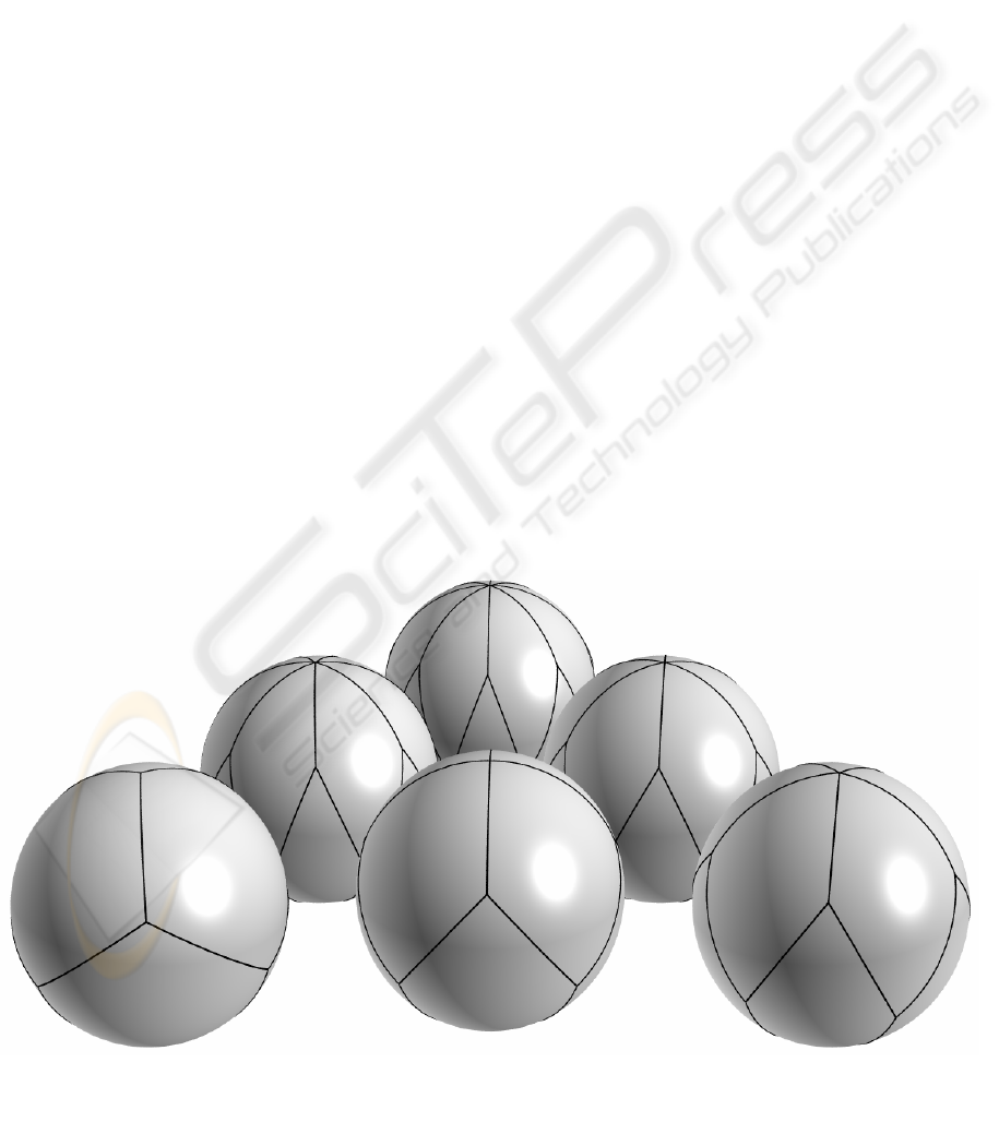
Consider a regular hexahedron (cube) inscribed in a
unit sphere. When its edges are projected to the
sphere, the sphere is tiled with a set of six diamonds.
This tiling set may be called a spherical cube.
In this tiling set, one of the vertices can be
chosen as the north pole. It is seen that three of the
tiles touch the north pole; the other three touch the
south pole. Instead of three diamonds sharing a pole,
any greater number of diamonds can share the north
pole, with the same number of diamonds sharing the
south pole. Such a tiling set is a member of an
infinite family of tiling sets. The first few members
of this family are shown in Figure 1.
As the number of diamonds increases, the small
vertex angles decrease and the large vertex angles
increase. For the tiling set of twelve diamonds, the
large vertex angle is 150°. Such a large vertex angle
may cause problems for intersections of geodesics
used for determining texel locations (as discussed in
Sections 5 and 6), so the use of this or larger tiling
sets in the family is not recommended. The
following section describes an alternative tiling set
of twelve diamonds with better geometric
characteristics. Thus only the first three members of
this family are judged to have practical use with
texturing; these three are in the foreground of Figure
1.
The spherical cube may be considered as an
alternative to the common single-tile latitude-
longitude technique described in Section 1. When
tiled spheres covered by the same total number of
texels are compared, the tiling set of six has the
advantages of a narrower range of texel areas and a
smaller maximum texel area (i.e., higher resolution).
The tiling set of eight diamonds provides slightly
higher resolution. This tiling set has no relation to a
regular polyhedron.
The tiling set of ten diamonds is a reasonable
compromise between simplicity of implementation
and high resolution for a given texture array size. Its
vertices are identical to those of an inscribed regular
icosahedron.
Figure 1: Members of an Infinite Family of Tiling Sets.
GRAPP 2007 - International Conference on Computer Graphics Theory and Applications
118
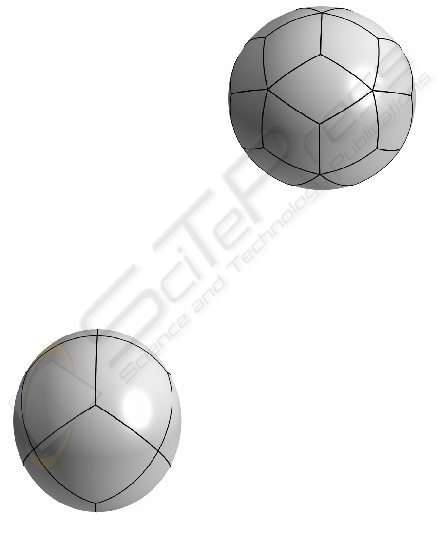
Figure 3: A Tiling Set of Thirty Diamonds.
Figure 2: A Tiling Set of Twelve Diamonds.
There is another infinite family of tiling sets. Its
members can be derived from members of the first
family by a simple transformation. For any tiling set
in the first family that has an odd number of
diamonds touching a pole, a cap on the side of the
sphere that is composed of almost half of the
diamonds is rotated almost 120° to produce a new
tiling set. This tiling set has a mirror image that is
also a member of this family. A tiling set in the first
family that has an even number of diamonds at a
pole has no corresponding member in the second
family. The spherical cube is a member of this
family but is a special case: the transformation
produces the same spherical cube, and the mirror
image is no different.
The only unique member of this family that may
have practical use with texturing is the tiling set of
ten, but it provides no specific advantage. This
family is described here only for completeness;
These two infinite families and the family described
in the following section include all diamond tiling
sets (Ueno and Agaoka, 2002).
4 THE FAMILY OF THREE
TILING SETS
For the first infinite family of tiling sets discussed
above, each non-polar vertex is shared by three
diamonds, and at each of these vertices are two
small vertex angles and one large vertex angle. In
the third family of tiling sets, at each vertex shared
by three diamonds all three vertex angles are large.
Thus, for the diamonds in these tiling sets, each
large vertex angle is 120°. Clearly, the spherical
cube is a member of this family as well. This family
has two other members.
The second member is a tiling set of twelve
diamonds; four diamonds surround each of the poles
and four diamonds ring the equator. This tiling set is
shown in Figure 2.
The third member is a tiling set of thirty
diamonds. Ten of the diamonds are centered on the
equator, and a ring of five diamonds lies between the
equatorial diamonds and each set of five polar
diamonds. This tiling set is appropriate for
applications requiring fine detail; for a given texture
array size, it provides the highest resolution of the
five tiling sets. This tiling set is shown in Figure 3.
5 DIAMOND COORDINATE
SYSTEM
The diamond coordinate system is a new coordinate
system that is based on geodesics and on the tiling
sets of diamonds. This coordinate system is
especially useful for textures on a sphere; it can
identify precisely the location of each texel on the
sphere’s surface. For any point feature on a sphere, it
can identify the texel containing the feature.
This system has three components, represented
as {d, u, v}. The first component, d, is an integer that
identifies one of the diamonds in a specific tiling set
(diamond identifiers may be assigned arbitrarily).
Thus, each tiling set has a different diamond
coordinate system. The specific tiling set being used
is assumed to be known by context.
TILING THE SPHERE WITH DIAMONDS FOR TEXTURE MAPPING
119
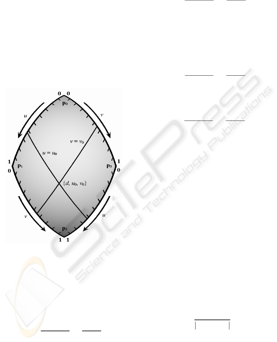
Figure 4: Diamond Coordinate System.
The second and third components of the diamond
coordinate system, u and v, identify a point on the
designated diamond by specifying two geodesics
that intersect at the point.
The u and v coordinates depend upon the four
vertices of the diamond. For each diamond, one of
the vertices with a small angle is designated as p
0
;
the other vertices are designated as p
1
, p
2
, and p
3
, in
counter-clockwise order. The other small angle is at
p
2
, and the large angles are at p
1
and p
3
. (Position
vectors are used to represent surface points; the
origin is at the center of the sphere.)
Each of the u and v coordinates ranges from 0 on
one edge of the diamond to 1 on the opposite edge.
Figure 4 illustrates the diamond coordinate system;
in this figure, u
0
and v
0
represent arbitrary constants.
Along edge p
0
-p
1
of the diamond, coordinate u
runs uniformly from 0 at vertex p
0
to 1 at vertex p
1
.
That is, a point on this edge can be expressed as a
spherical linear interpolation of the two vertices:
00 1
sin( ) sin( )
() .
sin( ) sin( )
u
SuS uS
u
SS
−
=+pp p
(1)
The parameter S is the arc length of the edge of the
diamond.
Similarly, along edge p
2
-p
3
, coordinate u runs
uniformly from 0 at p
3
to 1 at p
2
. A point on this
edge can be expressed as:
13 2
sin( ) sin( )
() .
sin( ) sin( )
u
SuS uS
u
SS
−
=+pp p
(2)
The locus of points with a given value of u is
defined to be the geodesic that connects the point
with the value of u on edge p
0
-p
1
with the point that
has the same value of u on edge p
2
-p
3
.
Along edge p
0
-p
3
of the diamond, coordinate v
runs uniformly from 0 at vertex p
0
to 1 at vertex p
3
.
A point on this edge can be expressed as:
00 3
sin( ) sin( )
() .
sin( ) sin( )
v
SvS vS
v
SS
−
=+pp p
Along edge p
1
-p
2
, coordinate v runs uniformly
from 0 at vertex p
1
to 1 at vertex p
2
. A point on edge
p
1
-p
2
can be expressed as:
11 2
sin( ) sin( )
() .
sin( ) sin( )
v
SvS vS
v
SS
−
=+pp p
The locus of points with a given value of v is
defined to be the geodesic that connects the point
with the value of v on edge p
0
-p
3
with the point that
has the same value of v on edge p
1
-p
2
.
A geodesic plane is conveniently specified by its
normal vector. With the convention that the normals
of the geodesic planes for constant u point in the
direction of increasing u, the normal of the geodesic
plane for a given u is:
10
() () () .
uuu
uuu=×npp (3)
Similarly, the normal of the geodesic plane for a
given v is:
01
() () () .
vvv
vvv
=
×npp
Specific values of u and v identify the point that
is the intersection of the two geodesic planes at the
surface of the sphere. The normals of the two
geodesic planes (u and v) are multiplied (vector
cross product) to yield the line that is the intersection
of the two planes. The intersection of this line and
the unit sphere is the point of interest. Thus,
Equation (4) converts a point from diamond
coordinates to Cartesian coordinates:
() ()
(,)
() ()
.
uv
uv
uv
uv
uv
×
=
×
nn
p
nn
(4)
To obtain diamond coordinates for any point p
on the unit sphere with known Cartesian
coordinates, the first step is to identify the diamond
(coordinate d) that contains the point. The scalar
(dot) product of a point p with the normal of a
geodesic plane indicates the side of the plane on
GRAPP 2007 - International Conference on Computer Graphics Theory and Applications
120

which p is located. Thus, point p is located on a
given diamond if this condition is true:
(0)0(1)0
(0) 0 (1) 0 .
uu
vv
•≥∧ •≤∧
•≥∧ •≤
npnp
npnp
(5)
If it is not known which diamond contains p, the
above condition can be tested for each diamond until
the correct one is found. If one or more of the dot
products is zero, p lies on an edge or a vertex
common to two or more diamonds.
In each tiling set, the edges of several diamonds
may lie on the same geodesic plane. As an
optimisation, these planes can be identified and used
to determine the diamond containing a point p
through fewer comparisons than implied by
Equation(5).
Points on edges and at vertices have multiple
representations. For example, a vertex that is
common to three diamonds has three coordinate
representations (one for each diamond).
For any point p on a diamond, a geodesic of
constant
u passes through the point. This relation is
expressed as:
() 0 .
u
u •=np
The value of
u that satisfies this equation is the u
coordinate of the point. Substituting the expression
for the normal from Equation(3), then substituting
the two edge points from Equation (1) and Equation
(2), leads to:
() () ()
2
tan ( ) tan( )
0 ,
uuu
uS uS•+•+•
=
ap bp cp
(6)
which is quadratic in tan(uS); the coefficient vectors
for Equation (6) are:
()
()
()
()
()
()
2
03
0213
12
03
0213
2
03
cos ( )
cos( )
,
2sin()cos()
sin( ) ,
sin ( ) .
u
u
u
S
S
SS
S
S
=×
−×+×
+×
=− ×
+×+×
=×
app
pp pp
pp
bpp
pp pp
cpp
If the point is in the relevant diamond [as
confirmed by Equation (5)], then u is obtained from
the quadratic root of Equation (6) that is between 0
and tan(S).
The value of the v coordinate is obtained in the
same manner, with p
1
and p
3
interchanged; the
coefficients are:
(
)
()
()
()
()
()
2
01
02 31
32
01
02 31
2
01
cos ( )
cos( )
,
2 sin( )cos( )
sin( ) ,
sin ( ) ,
v
v
v
S
S
SS
S
S
=×
−×+×
+×
=− ×
+×+×
=×
app
pp pp
pp
bpp
pp pp
cpp
and the quadratic equation is:
(
)
(
)()
2
tan ( ) tan( )
0 .
vvv
vS vS
•
+• +•
=
ap bp cp
(7)
Thus, for each diamond, there are two sets of
constant vectors (a
u
, b
u
, c
u
and a
v
, b
v
, c
v
) that are
used to obtain quadratic coefficients from a point p.
Therefore, Equation (4) converts from diamond
coordinates to Cartesian coordinates, and Equations
(5), (6) and (7) convert from Cartesian coordinates
to diamond coordinates.
The conversions in Equations (6) and (7) also
underlie the necessary texture mapping function
discussed generally in Section 1 and specifically for
diamonds in Section 6.
The conversion from Cartesian coordinates to
diamond coordinates adds significant capability to
the diamond coordinate system, as an interactive
graphics application illustrates. The screen
coordinates corresponding to a mouse click can be
converted to a ray in the view frustum. The
intersection of this ray with a sphere is a point with
determinable Cartesian coordinates, which can be
converted to diamond coordinates to identify a texel
in a texture array. The same considerations apply to
ray-tracing.
6 SUBDIVIDING DIAMONDS TO
TEXELS
A grid of geodesics of constant u and of constant v
subdivides a diamond into an array of (non-
equilateral) sub-diamonds. Typically the values of u
and v for a grid would be chosen to be equally
spaced, and spaced such that there is a one-to-one
correspondence between the sub-diamond
quadrilaterals and the texture array texels.
Thus, the diamond coordinates u and v are
identical to the texture image coordinates u and v
described in Section 1; the necessary texture
mapping function is the identity function [as is
usually true also for parametric surface patches
(Foley et al. 1996; Watt and Watt, 1992)].
TILING THE SPHERE WITH DIAMONDS FOR TEXTURE MAPPING
121
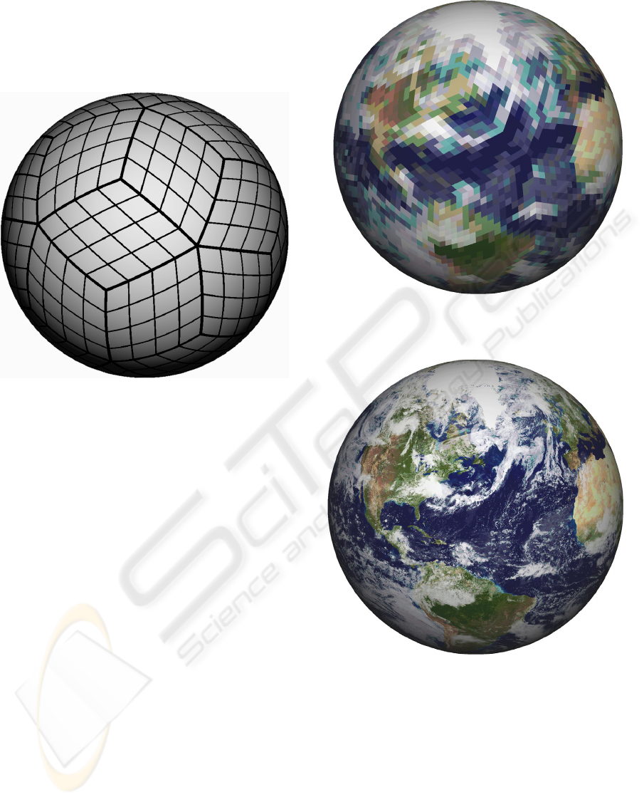
Figure 7: Sphere Textured with the Tiling Set of Thirty;
n = 256.
Figure 6: Sphere Textured with the Tiling Set of Thirty;
n = 16.
Figure 5: Sphere with Tiling Set of Thirty; n = 4.
For a grid of equally-spaced subdivisions, an
important parameter is the number of sub-diamonds
on each side of a diamond; this number is designated
here as n. This number can be any positive integer,
but is typically a power of 2, following from texture
array sizes.
Figure 5 shows the tiling set of thirty with
diamonds subdivided by geodesics of constant u and
v. For illustrative purposes, each diamond has four
sub-diamonds on a side. Graphics systems
commonly have an optimum size for texture arrays;
256 pixels on each side are probably a minimum for
practical use. As is discussed in Section 7, a smaller
number of subdivisions can be useful for other
purposes.
Figure 6 shows a textured sphere with the tiling
set of thirty; each diamond has 16 sub-diamonds on
a side (thus, each texture array is 16x16). Many of
the individual texels are clearly visible; with
reference to Figure 5, various diamond vertices can
be located.
As high resolution is a desirable goal, Figure 7
shows the same textured sphere with the same tiling
set as Figure 6, but each diamond has 256 sub-
diamonds on a side. A sphere textured with any of
the other four tiling sets and with the same texture
array size would not appear noticeably different,
unless the viewpoint were extremely close to the
sphere.
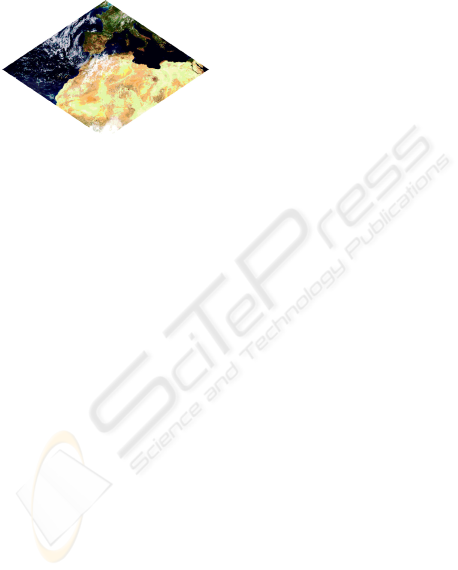
Figure 8 shows the texture array associated with
one of the diamonds of Figure 7. Although the
texture array is square, the rhombic arrangement
shown gives the best planar representation of its
image. This arrangement requires a linear
transformation (skew and rotation) of the u and v
coordinates and is for visualization of a texture array
only; it is not an integral part of the texture mapping.
GRAPP 2007 - International Conference on Computer Graphics Theory and Applications
122
7 RENDERING WITH
TRIANGLES
For fast animation, curved surfaces are often
approximated by meshes of polygons, usually
triangles. Subdivision of diamonds leads readily to
such an approximation. When the four edges of a
sub-diamond are replaced by line segments, and the
opposite vertices with large angles are connected by
a line segment, the result is a pair of (non-coplanar)
triangles.
Figure 5 serves as an example because it could
have been rendered this way. Each of the 16 sub-
diamonds on a diamond can be approximated by a
pair of triangles. This example would lead to a
sphere approximated by a mesh of 960 triangles.
Thus, spherical diamonds can be subdivided to
various levels for different purposes. At the finest
level of subdivision, the resulting sub-diamonds
correspond to texels. At a coarser level of
subdivision, the sub-diamonds correspond to triangle
pairs for fast rendering through a mesh of triangles.
ACKNOWLEDGEMENTS
Texture arrays used in the colour figures were
derived from the NASA image “The Blue Marble:
Land Surface, Ocean Color, Sea Ice and Clouds”
available online at www.visibleearth.nasa.gov.
Figures 1, 2, and 3 were generated with POV-Ray,
available online at www.povray.org.
REFERENCES
Borgefors, G., 1992. A hierarchical ‘square’ tessellation of
the sphere, Pattern Recognition Letters, 13, 183-188.
Dutton, G. H., 1999. A hierarchical coordinate system for
geoprocessing and cartography, Lecture Notes in
Earth Sciences, Vol. 79, Berlin: Springer-Verlag.
Foley, J. D., van Dam, A., Feiner, S. K., & Hughes, J. F.,
1996. Computer graphics: Principles and practice,
Reading, MA: Addison-Wesley, pp. 741-744.
Fuller, R. B., 1946. US Patent No. 2 393 676.
Giraldo, F. X., 2001. A spectral element shallow water
model on spherical geodesic grids, International
Journal for Numeric Methods in Fluids, 35, 869-901.
Górski, K. M., Hivon, E., Banday, A. J., Wandelt, B. D.,
Hansen, F. K., Reinecke, M., & Bartelmann, M., 2005.
HEALPix: a framework for high-resolution
discretization and fast analysis of data distributed on
the sphere, The Astrophysical Journal, 622, 759–771.
Gray, R. W., 1995. Exact transformation equations for
Fuller’s world map, Cartographica, 32 (3), 17-25.
Heckbert, P. S., 1986. Survey of texture mapping, IEEE
Computer Graphics and Applications, 6 (6), 56-67.
Nielson, G. M., 1993. Modeling and visualizing
volumetric and surface-on-surface data, in H. Hagen,
H. Mueller, & G. M. Nielson, (Eds.), Focus on
scientific visualization (pp. 191-242), New York:
Springer-Verlag.
Pottman, H., & Eck, M., 1990. Modified multiquadric
methods for scattered data interpolation over a sphere,
Computer Aided Geometric Design, 7, 313-321.
Ramaraj, R., 1986. Interpolating scattered data on a
sphere, master’s thesis, Computer Science Dept.,
Arizona State Univ.
Renka, R. J., 1984. Interpolation of data on the surface of
a sphere, ACM Trans. on Mathematical Software, 10,
417-436.
Ueno, Y., & Agaoka, Y., 2002. Classification of the tilings
of the 2-dimensional sphere by congruent triangles,
Hiroshima Math. J., 32, 463–540.
Watt, A. H., & Watt, M., 1992. Advanced animation and
rendering techniques: Theory and practice, Reading,
MA: Addison-Wesley, pp. 179-186.
White, D., Kimerling, J., & Overton, W. S., 1992.
Cartographic and geometric components of a global
sampling design for environmental monitoring,
Cartography and Geographic Information Systems,
19
, 5-22.
Wickman, F. E., Elvers, E., & Edvarson, K., 1974. A
system of domains for global sampling problems,
Geografiska Annaler, Series A: Physical Geography,
56, 201-212.
Figure 8: A Texture Array (256x256), Skewed and
Rotated, for a Diamond in the Tiling Set of Thirty.
TILING THE SPHERE WITH DIAMONDS FOR TEXTURE MAPPING
123
