
DIFFRACTION MODELING FOR INTERACTIVE VIRTUAL
ACOUSTICAL ENVIRONMENTS
Bill Kapralos
Faculty of Business and Information Technology, University of Ontario Institute of Technology
200 Simcoe Street North, Oshawa, Ontario, Canada, L1H 7K4
Michael Jenkin
Dept. of Computer Science and Engineering, Centre for Vision Research, York University. Toronto, Ontario, Canada, M3J 1P3
Evangelos Milios
Faculty of Computer Science, Dalhousie University. Halifax, Nova Scotia, Canada, B3H 1W5
Keywords:
Sonel mapping, acoustical diffraction modeling, virtual environments.
Abstract:
Since the dimensions of many of the objects/surfaces encountered in our daily lives are within an order of mag-
nitude of the wavelength of audible sounds, diffraction is an elementary means of sound propagation. Despite
its importance in the real-world, diffraction effects are often overlooked by acoustical modeling methods lead-
ing to a degredation in immersion or presence. This paper describes an acoustical diffraction method based on
the Huygens-Fresnel principle. The method is simple and efficient allowing it to be incorporated in interactive
acoustical environments including virtual environments. Experimental results are presented that illustrate the
performance and effectiveness of the method and its conformance to theoretical diffraction models.
1 INTRODUCTION
Diffraction refers to the “bending mode” of sound
propagation whereby sound waves go (“bend”)
around an obstacle that lies directly in the line of
straight propagation between the sound source and re-
ceiver. Diffraction is dependent on both wavelength
and obstacle/surface size, increasing as the ratio be-
tween wavelength and obstacle size is increased (Cre-
mer and M
¨
uller, 1978). Since the dimensions of many
of the objects/surfaces encountered in our daily lives
are within an order of magnitude as the wavelength
of audible sounds, diffraction is an elementary means
of sound propagation, especially when there is no di-
rect path between the sound source and the receiver
(Tsingos et al., 2002).
Diffraction is a phenomenon of all wave propa-
gation including sound and light waves and several
approaches have been developed to model its effects.
One such approach is the Huygens-Fresnel principle,
originally formulated by Christian Huygens in 1678
and later modified and extended by Augustin Fresnel.
Although it is a rather simple approach, it can sat-
isfactorily model a large number of diffraction con-
figurations in a simple and efficient manner. The
Huygens-Fresnel principle is based on the assump-
tion that at every time instant, every point on a pri-
mary wavefront of an emitted sound can be thought
of as a continuous emitter of secondary wavelets
(sources) and these secondary wavelets combine to
produce a new wavefront in the direction of propaga-
tion. This assumption fits nicely with particle-based
acoustical modeling methods whereby the acoustics
of an environment is determined by emitting sound
“particles” from a sound source and tracing them
through the environment. One such particle-based
method is sonel mapping (Anonymous, 2006). Sonel
mapping is a two-pass probabilistic, “particle-based”,
acoustical modeling method inspired by the popu-
lar image synthesis photon mapping method (Jensen,
2001). Sonel mapping models the propagation of
sound within an environment, taking into account
the relevant acoustical phenomena experienced by a
propagating sound in an efficient manner for use in
dynamic virtual environments. This paper describes
an efficient acoustical diffraction modeling technique
based on the Huygens-Fresnel principle. The tech-
nique described is incorporated within the sonel map-
241
Kapralos B., Jenkin M. and Milios E. (2007).
DIFFRACTION MODELING FOR INTERACTIVE VIRTUAL ACOUSTICAL ENVIRONMENTS.
In Proceedings of the Second International Conference on Computer Graphics Theory and Applications - AS/IE, pages 241-248
DOI: 10.5220/0002075802410248
Copyright
c
SciTePress

ping method although it could easily be incorporated
into other geometric-based acoustical modeling meth-
ods.
The remainder of this paper is organized as fol-
lows. Section 2 reviews several available acousti-
cal diffraction methods for virtual environment ap-
plications. Section 3 provides a brief introduction to
the optics-based Huygens-Fresnel principle followed
by a detailed description of the acoustical diffraction
method. Section 4 provides the results of experiments
conducted to demonstrate the effectiveness of the de-
veloped acoustical diffraction modeling method. Fi-
nally, concluding remarks are given in Section 5.
2 BACKGROUND
The two major approaches to computational acousti-
cal modeling (e.g., estimating the room impulse re-
sponse) are (Funkhouser et al., 2004) wave-based
modeling whereby numerical solutions to the wave
equation are sought and geometric modeling whereby
sound is approximated as a ray phenomenon and
traced through the scene. Although wave-based meth-
ods can account for non-specular reflection phenom-
ena, they are very expensive computationally mak-
ing them impractical for all but very simple, static
environments. Geometric modeling, and in partic-
ular ray-based approaches are the most widely used
due to their simplicity and computational feasibility.
Geometric modeling methods such as image sources
(Allen and Berkley, 1979) and ray tracing (Krokstad
et al., 1968; Kulowski, 1985) assume that sound is
a ray phenomena (Cremer and M
¨
uller, 1978) and
model all interactions between sound rays and ob-
jects/surfaces as specular. As a result, they typically
ignore the wavelength of sound and any phenom-
ena associated with it including diffraction (Calamia
et al., 2005).
That being said, a limited number of research ef-
forts have investigated acoustical diffraction model-
ing. The beam tracing approach of Funkhouser et al.
(2003) for acoustical modeling/rendering includes an
extension capable of approximating diffraction. Their
frequency domain method is based on the uniform
theory of diffraction (UTD) (Keller, 1962). Validation
of their approach by Tsingos et al. (2002) involved a
comparison between actual impulse responses (e.g.,
the energy reaching a receiver over a period of time)
measured in a simple enclosure (the “Bell Labs Box”)
and the impulse responses obtained by simulating the
enclosure. Tsingos et al. (2002) observed that their
combined technique was the first instance to use a
physically-based diffraction model to produce inter-
active rate sounds in a complex virtual environment.
Tsingos and Gascuel (1997) developed an occlu-
sion and diffraction method that utilizes computer
graphics hardware to perform fast sound visibility cal-
culations that can account for specular reflections, ab-
sorption, and diffraction caused by partial occluders.
Diffraction is approximated by computing the fraction
of sound that is blocked by obstacles (occluders) be-
tween the path from the sound source to the receiver
by considering the amount of volume of the first Fres-
nel ellipsoid blocked by the occluders. Rendering of
occluders is performed from the receiver’s position.
A count of all pixels not in the background is taken
and pixels that are “set” (e.g., not in the background)
correspond to occluders. Their approach is near-real-
time using graphics hardware to operate in an efficient
manner.
In later work, Tsingos and Gascuel (1998) intro-
duced another occlusion and diffraction method based
on the Fresnel-Kirchoff optics-based approximation
to diffraction. As with the Huygens-Fresnel approx-
imation, the Fresnel-Kirchoff approximation is based
on Huygens’ principle. The total unoccluded sound
pressure level at some point p in space is determined
by calculating the sound pressure of a small differ-
ential area dS and integrating over the closed sur-
face enclosing p. After determining the total unoc-
cluded sound arriving at point p from a sound source,
diffraction and occlusion effects are accounted for by
computing an occlusion depth-map of the environ-
ment between the sound source and the receiver (lis-
tener) using computer graphics hardware to permit
real-time operation. Once this depth-map has been
computed, the depth of any occluders between the
sound source and the receiver can be obtained from
the Z-buffer whereby “lit” pixels correspond to oc-
cluded areas. The diffraction integral described by the
Fresnel-Kirchoff approximation is then approximated
as a discrete sum of differential terms for every oc-
cluded pixel in the Z-buffer. Comparisons for several
configurations with obstacles of infinite extent made
between their method and between boundary element
methods (BEMs), produced “satisfactory quantitative
results” (Tsingos and Gascuel, 1998).
3 DIFFRACTION MODELING
The Huygens-Fresnel principle states that every point
on the primary wavefront can be thought of as a
continuous, direction dependent emitter of secondary
wavelets (sources) that combine to produce a new
wavefront in the direction of propagation (Hecht,
2002). These secondary wavelets are emitted in a
GRAPP 2007 - International Conference on Computer Graphics Theory and Applications
242

direction dependent manner, essentially scaled by an
obliquity or inclination factor K(θ) as
K(θ) =
1
2
(1 + cos(θ)) (1)
where θ is the angle between the receiver and the
direction of propagation of the primary wavefront
(Hecht, 2002). This expanding wavefront can be di-
vided into a number of ring-like regions, collectively
known as Fresnel zones (Hecht, 2002). The bound-
ary of the i
th
Fresnel zone (Z
i
) corresponds to the
intersection of the wavefront with a sphere of radius
r
◦
+ iλ/2 centered at the receiver where, r
◦
is equal
to the distance between the receiver and the expand-
ing wavefront after it has traversed a distance of ρ
from the sound source. In other words, the distance
from the receiver to each adjacent Fresnel zone dif-
fers by half a wavelength (λ/2). Each Fresnel zone
contains secondary sources that are assumed to emit
their energy in phase with the primary wave. The
secondary sources within each Fresnel zone i emits
energy collectively equal to E
i
and a portion of this
energy may reach the receiver. By summing the con-
tribution of energy reaching the receiver from each of
the Fresnel zones, the total energy leaving the sound
source and reaching the receiver (E
total
) can be calcu-
lated. It can be shown that the total energy is approx-
imately equal to half the energy of the first Fresnel
zone reaching the receiver (Hecht, 2002) or, mathe-
matically E
total
≈ |E
1
|/2. A detailed mathemati-
cal derivation of the Huygens-Fresnel principle is pre-
sented by Hecht (2002).
3.1 Huygens-Fresnel Acoustical
Diffraction Modeling
In the sonel mapping method (Anonymous, 2006),
at each sound source, sonels are emitted and traced
through the environment while recording their inter-
action with any surfaces/objects they may encounter.
Upon encountering a surface, a decision is made as
to whether the sound particle (known as a sonel)
will be reflected specularly or diffusely, diffracted
or completely absorbed (the decision is made prob-
abilistically based on various parameters including
frequency, distance to an edge, etc. using a Russian
roulette strategy (Kapralos et al., 2005)). Whether or
not the sonel is actually incident on the edge itself or
close to the edge, if the sonel is to be diffracted, its
position is assumed to be on the edge (p
edg e
). Since
the position of both the sound source and p
edg e
are
known, the distance between them r
se
can be deter-
mined. The radius of the primary wavefront is then
set to this distance (e.g., ρ = r
se
- see Figure 1).
S (source)
R (receiver)
φ
ρ sinφ
First Fresnel
zone Z
1
First ray-sphere
intersection point
(p
0
)
Second ray-sphere
intersection point
r
r + λ/2
ρ
Imaginary line
between source
and receiver
Secondary source
position in the first
Fresnel zone (p
1
)
Figure 1: Determining the position of a secondary source
within the first Fresnel zone.
Since ρ is the distance between the position of the
sound source and p
edg e
, p
edg e
must be located on the
surface of the wavefront and within one of the Fres-
nel zones (the “initial” Fresnel zone) denoted by Z
init
and calculated as
Z
init
=
r
init
− r
◦
λ
+ 0.5
. (2)
Here r
init
is the distance between the receiver and
p
edg e
and r
◦
is the distance between the receiver and
primary wavefront given as r
◦
= r
SR
− ρ where, r
SR
is the distance between the sound source and the re-
ceiver. Although p
edg e
may lie anywhere within Z
init
and not necessarily on its boundary, it is assumed that
the obliquity factor is constant throughout the entire
zone (Hecht, 2002) and therefore, its position within
the zone does not matter. Given the position of the
secondary source in Z
init
, the position of a secondary
source within the first Fresnel zone (Z
1
) can be deter-
mined. Referring to Figures 1 and 2, this is accom-
plished in two steps:
1. Rotate p
edg e
such that it lies directly on the (imag-
inary) line between the sound source and receiver.
This essentially moves p
edg e
to a new position de-
noted by p
◦
.
2. Move p
◦
to yet another new position (p
1
) within
the first Fresnel zone.
Determining p
◦
: The original position p
edg e
that
lies within Z
init
is rotated such that it lies directly
on the (imaginary) line between the sound source and
receiver. This can be performed using a series of rota-
tions about the central axes. However, this is actually
accomplished by taking the (first) point of intersection
(denoted by p
◦
) between the sphere representing the
initial wavefront and a ray (normalized vector) whose
origin is the receiver position and whose direction is
towards the sound source.
DIFFRACTION MODELING FOR INTERACTIVE VIRTUAL ACOUSTICAL ENVIRONMENTS
243

Z
Y
X
ρ
y
x
z
Sphere representing
initial wavefront of
radius ρ.
Figure 2: Spherical coordinates.
Determining p
1
: Once the intersection point (p
◦
)
has been determined, it is moved to the first Fresnel
zone. Referring to Figures 1 and 2, angles θ (the hor-
izontal angle of p
◦
relative to the sound source) and φ
(the vertical angle of p
◦
relative to the sound source)
are calculated as
θ = tan
−1
x
p
− x
s
z
p
− z
s
, φ = cos
−1
(
y
p
− y
s
ρ
)
(3)
where (x
s
, y
s
, z
s
) and (x
p
, y
p
, z
p
) are the spatial co-
ordinates of the sound source and p
◦
respectively. As
with p
◦
, the position of the secondary source in the
first Fresnel zone (p
1
) also lies on the surface of the
sphere corresponding to the initial propagating wave-
front of radius ρ. The difference in distance between
adjacent Fresnel zones and the receiver is λ/2. There-
fore, the difference in distance (r
diff
) between the
receiver and p
◦
and the receiver and the secondary
source in the first Fresnel zone p
1
must also be λ/2.
Position p
1
is determined iteratively until r
diff
is
within of λ/2. Once the position of a secondary
source within the first Fresnel zone (Z
1
) has been de-
termined, the energy (E
1
) reaching the receiver from
Z
1
can be calculated as (Hecht, 2002)
E
1
= (−1)
1+1
2K
1
(θ)E
A
ρλ
(ρ + r
◦
)
sin[ωt − k(ρ + r
◦
)]
=
2K
1
(θ)E
A
ρλ
(ρ + r
◦
)
sin[ωt − k(ρ + r
◦
)]. (4)
Here K
1
(θ) is the obliquity factor of Z
1
and r
◦
is
the distance between the receiver and the expanding
wavefront after it has traversed a distance of ρ from
the sound source. t is the time taken for a secondary
source in Z
1
to reach the receiver, k = 2πλ is the
wave-number and E
A
is the energy per unit area of
the secondary sources within a differential area of the
Fresnel zone (see (Hecht, 2002)). Adding terms to ac-
count for absorption of sound energy by the medium
(air), Equation 4 becomes
E
1
= K
1
(θ) × E
◦
e
−m(ρ+r
◦
)
× sin[ωt − k(ρ + r
◦
)]
(5)
Source
Receiver
Occluder
Initial
wavefront
Blocked (non-
visible) rays
Fresnel
zone
Non-blocked
(visible) rays
Figure 3: Sampling a Fresnel zone in the presence of an
occluding edge using ray-casting.
where E
◦
is the ray energy and m is the air absorp-
tion constant that varies as a function of the condi-
tions of the air itself. As presented above, the energy
reaching the receiver from the first Fresnel zone can
be calculated assuming an obstruction-free path be-
tween each zone and the receiver (e.g., the first zone
is completely visible to the receiver). Edge effects are
accounted for by considering the visibility weighting
v
1
for the first zone Z
1
relative to the receiver using
ray casting. n
rays
rays are emitted from the receiver
to uniformly sampled positions within Z
1
. A check
is made to determine whether each sampled position
is visible relative to the receiver (see Figure 3). The
visibility weighting is determined by considering the
number of visible (non-blocked) rays (n
v is
) relative
to the total number of emitted rays (N
v is
) or, mathe-
matically, v
1
= n
v is
/N
v is
. Taking edge effects into
account, the total energy reaching the receiver from
the first Fresnel zone Z
1
is given as
E
1
= v
1
×K
1
(θ)×E
◦
e
−m(ρ+r
◦
)
×sin[ωt
1
−k(ρ+r
◦
)]
(6)
where t
1
= (r
◦
+ λ/2)/v
s
is the time taken for
the secondary sources within the first Fresnel zone to
reach the receiver and v
s
= 343m · s
−1
is the speed
of sound in air.
3.2 Considering All Fresnel Zones
Rather than considering the first Fresnel zone only,
the entire sphere representing the initial wavefront
emitted from the sound source is divided into differ-
ent Fresnel zones. The energy arriving at the receiver
from each of these Fresnel zones is summed to deter-
mine the amount of energy reaching the receiver. The
total number of zones (N
zones
) is given by
N
zones
=
2ρ
(λ/2)
. (7)
To account for diffraction effects, a visibility factor
for each Fresnel zone is introduced. The visibility
factor (denoted by v
i
), represents that fraction of the
i
th
Fresnel zone visible relative to the receiver. As
with the first zone-only approximation previously de-
scribed, the edge position p
edg e
is assumed to lie
GRAPP 2007 - International Conference on Computer Graphics Theory and Applications
244

on the sphere representing the initial wavefront and
within a particular Fresnel zone Z
init
. Given the po-
sition of the secondary source in Z
init
, the position of
a secondary source within the first Fresnel zone (p
1
)
can be determined using the two step process previ-
ously described. Upon determining p
1
, simple ge-
ometry allows for the position of a secondary source
within Fresnel zone Z
2
to be determined. The same
reasoning can be applied to finding the position of a
secondary source within the third Fresnel zone and
subsequent zones until the position of a secondary
source within all the Fresnel zones considered has
been found (the mathematics describing this process
are developed in Section 3.2.1). Once the position of
a secondary source within a zone Z
i
has been deter-
mined, the energy reaching the receiver from Z
i
can
be calculated using Equation 5.
Edge effects are accounted for by considering the
visibility weighting v
i
of each zone Z
i
relative to the
receiver, using ray casting as described in the previous
section. Taking edge effects into account, the total
energy reaching the receiver from zone Z
i
is given as
E
i
= v
i
× (−1)
i+1
× K
i
(θ) × E
◦
e
−m(ρ+r
◦
)
×
sin[ωt
i
− k(ρ + r
◦
)] (8)
where t
i
= (r
◦
+ iλ/2)/v
s
is the time taken for the
secondary sources within Fresnel zone i to reach the
receiver. The total energy E
total
reaching the receiver
from the sound source taking edge effects into consid-
eration is determined by summing the energy reach-
ing the receiver from each of the N Fresnel zones
E
total
= (v
1
× E
1
) + (v
2
× E
2
) + · · · + (v
N
× E
N
).
(9)
3.2.1 Finding the Position of a Secondary Source
Within a Fresnel Zone
The distance between secondary sources in adjacent
zones (e.g., between zones Z
1
and Z
2
) is λ/2. Refer-
ring to Figure 1
dS = ρdϕ2π(ρ sin ϕ). (10)
Applying the law of cosines,
r
2
= ρ
2
+ (ρ + r
0
)
2
− 2ρ(ρ + r
0
) cos ϕ (11)
where r is the distance between the receiver and the
secondary source in a particular Fresnel zone. By re-
arranging Equation 11, an expression for φ, the angle
between the line connecting the sound source and re-
ceiver and the line from the sound source to the sec-
ondary source, can be determined
cosφ =
r
2
− ρ
2
+ (ρ + r
◦
)
2
−2ρ(ρ + r
◦
)
. (12)
Receiver
Source
Sphere representing
initial wavefront
Secondary source
in first Fresnel zone
Secondary source in
second Fresnel zone
Figure 4: Sampling a secondary source within a particular
Fresnel zone considering a 63Hz sound source.
By differentiating Equation 11 above, an expression
for the value of 2rdr can be obtained (e.g., 2rdr =
2ρ(ρ+r
◦
) sin(ϕ)dϕ) where dr is the difference in dis-
tance between the receiver and the secondary sources
between adjacent differential areas dS. Since a partic-
ular Fresnel zone is comprised of several differential
areas, the value of dr is not necessarily equal to λ/2.
Here dr is set to a value of λ/2 thus representing an
adjacent Fresnel zone as opposed to an adjacent dif-
ferential area within a zone. With the values of both
dr and φ, an expression for dφ is obtained
dφ =
2rdr
2ρ(ρ + r
◦
)sinφ
. (13)
Referring to Figure 1, since the elevation angle θ and
the radius of the initial wavefront ρ remain constant
the position of a secondary source in the adjacent
zone can now be determined. This is accomplished
by solving for each of its x,y,z coordinates using the
equations for the Cartesian coordinates (see Figure
2) of the sphere along with the previously computed
value of dφ
x = x
s
+ (ρsin(θ)sin(φ + dφ)) (14)
y = y
s
+ (ρsin(θ)cos(φ + dφ)) (15)
z = z
s
+ (ρcos(θ)). (16)
Figure 4 provides a graphical illustration of the sam-
pling of a secondary source in each Fresnel zones for
a 63Hz sound source.
4 EXPERIMENTAL VALIDATION
A series of experiments are presented that describe the
effectiveness of the developed acoustical diffraction
modeling method.
4.1 Model Correctness
In this experiment the validity of the energy reach-
ing a receiver as calculated using the Huygens-Fresnel
principle is examined. This is accomplished by con-
sidering the energy reaching the receiver from the
sound source using both Huygens-Fresnel implemen-
tations (one Fresnel zone only and all Fresnel zones)
with the visibility of the first Fresnel zone assumed
DIFFRACTION MODELING FOR INTERACTIVE VIRTUAL ACOUSTICAL ENVIRONMENTS
245

(55m,25m,50m)
(105m,0m,50m)
(105m,50m,50m)
Source
Receiver
Receiver
Receiver “y”
coordinate
ranges from
0m to 50m
(65m,25m,50m)
Edge (p
edge
)
10m 40m
Figure 5: Room set-up used in the correctness of the acous-
tical diffraction method simulation.
to be one and comparing the results with the results
obtained using the harmonic spherical wave model
(Hecht, 2002)
E =
E
◦
ρ
cos(ωt
0
− kρ). (17)
Here, E is the energy arriving at the receiver E
◦
is the
energy of the source at time t = 0. ρ is the radius of
the sphere representing the initial wavefront and set to
a value equal to the distance between the sound source
and the position on the edge (P
edg e
). t
0
is the time
it takes for the wave to propagate a distance ρ (e.g.,
t
0
= ρ/343m · s
−1
). As shown in Figure 5, the sound
source and edge position (p
edg e
) remained stationary
while the receiver’s position (the “y” coordinate) was
varied in unit increments from y = 0m to y = 50m.
The experiment considered the following frequencies:
63Hz, 125Hz, 250Hz, 500Hz, 1kHz, 2kHz, 4kHz and
8kHz. The experiment was repeated using the acous-
tical diffraction models where only the first Fresnel
zone was considered and where all Fresnel zones were
considered. A graphical summary of the results is
presented in Figure 6 where the average percentage
difference (e.g., the difference between the energy as
simulated using sonel mapping and the energy as cal-
culated with the harmonical spherical wave model av-
eraged over all 51 positions for each frequency) is
plotted against frequency for each of the two scenar-
ios considered. The smallest and largest average per-
centage difference for the diffraction implementation
whereby only the first Fresnel zone was considered
are small, 0.99 and 1.02 respectively. Despite ignor-
ing the energy of all zones other than the first, this
implementation provides a reasonable approximation.
In contrast, the range of percentage differences for the
diffraction implementation where all Fresnel zones
were considered is larger, ranging from 0.23 to 5.88
and typically increase with increasing frequency. This
increase in percentage difference may be due to nu-
merical errors associated with locating a secondary
source in each of the Fresnel zones. As frequency
increases, the number of Fresnel zones also increases
thus, any errors associated with locating a secondary
source in a particular Fresnel zone propagates through
(e.g., locating a secondary source in Fresnel zone i
Frequency (Hz)
0 2000 4000 6000 8000
Percent Difference
0
2
4
6
All Fresnel zones
First Fresnel zone only
Percent Difference = 0
Figure 6: Graphical summary of the results for the correct-
ness of the acoustical diffraction method simulation. Av-
erage percentage difference between the energy as simu-
lated using both Huygens-Fresnel implementations and the
energy as calculated with the harmonical spherical wave
model averaged over all 51 positions for each frequency)
along with error bars (standard deviation) as a function of
frequency.
requires the position of a secondary source in zone
i − 1). Therefore, an error in the position of the sec-
ondary source in zone i − 1 may propagate and there-
fore, result in an incorrect secondary source position
in zone i.
4.2 First Fresnel Zone Visibility as a
Function of Receiver Height
In this simulation, the visibility of the first Fresnel
zone relative to the receiver and the sound level at
the receiver was examined as a function of frequency.
A stationary sound source was positioned at coordi-
nates (40m, 25m, 50m) and the edge position (p
edg e
)
was set at coordinates (50m, 25m, 50m). The re-
ceiver was positioned at three locations: i) below the
edge position at coordinates (110m, 24m, 50m) (Fig-
ure 7(a)), ii) at the same height as the edge posi-
tion at coordinates (110m, 25m, 50m) (Figure 7(b)),
and iii) above the edge position at coordinates (110m,
26m, 50m) (Figure 7(c)). For each of the three sce-
narios, the energy reaching the receiver was calcu-
lated for each of the following frequencies: 63Hz,
125Hz, 250Hz, 500Hz, 1000Hz, 2000Hz, 4000Hz
and 8000Hz. Frequency dependent attenuation of the
sound by the air was ignored to allow for the fre-
quency dependent diffraction effects to be examined.
The purpose of this experiment is to compare the
Huygens-Fresnel diffraction implementation with the
theoretical diffraction model that states diffraction in-
creases with increasing frequency (decreasing wave-
length) for various sound source, edge and receiver
configurations. Since the visibility of the first Fresnel
GRAPP 2007 - International Conference on Computer Graphics Theory and Applications
246
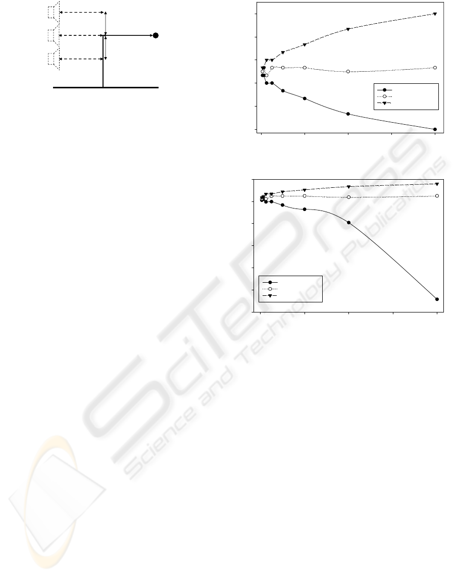
Receiver
Source Edge
60m10m
1m
1m
(a)
(b)
(c)
Figure 7: Set-up for the first Fresnel zone visibility as a
function of receiver height simulation. With respect to the
y-axis, receiver is: (a) below the edge position, (b) at same
height as the edge position and (c) above the edge position.
zone is directly related to the amount of energy reach-
ing the receiver via diffraction, frequency vs. visibil-
ity is used as a measure of performance. A graphical
summary of the results for each of the three scenar-
ios is provided in Figures 8. In Figure 8(a), the visi-
bility of the first Fresnel zone relative to the receiver
is plotted as a function of frequency. In Figure 8(b),
receiver level is plotted as a function of frequency.
In both plots, the filled circles and solid line repre-
sents the first scenario where the receiver is below
the edge position. The open circle and short dashed
line represents the scenario where the receiver is at
the same height as the edge position (and above the
sound source) and the triangle and long dashed line
represents the scenario where the receiver is above
the edge position. The results for the configuration
considered in the first scenario (e.g., receiver below
the edge position) are as expected. In particular, the
visibility of the first Fresnel zone is inversely propor-
tional to frequency whereby, as frequency increases,
visibility decreases. The decrease in visibility is due
to a decrease in the size of the first Fresnel zone and
this results in a decrease in the sound energy reach-
ing the receiver. As a result, as frequency increases,
the sound energy reaching the receiver decreases, thus
conforming to the theoretical model that predicts an
increase in diffraction as frequency decreases (Cre-
mer and M
¨
uller, 1978). In particular, the visibility
of the first Fresnel zone is used to scale the unoc-
cluded energy reaching the receiver after being emit-
ted from the sound source. Since there is a direct re-
lationship between visibility and energy reaching the
receiver (e.g., as visibility increases, the energy reach-
ing the receiver increases as well), visibility will in-
crease with increasing frequency.
The results of the second scenario where the re-
ceiver was positioned at the same height as the edge
position are also as expected. The visibility is ap-
proximately 0.5 irrespective of frequency indicating
that half of the zone is visible relative to the receiver.
Finally, in the third scenario where the height of the
receiver is greater than the height of the edge, visibil-
Frequency (Hz)
0 2000 4000 6000 8000
Visibility ( n
vis
/ N
vis
)
0.0
0.2
0.4
0.6
0.8
1.0
S(y) = R(y) = 24
S(y) = R(y) = 25
S(y) = R(y) = 26
(a) Frequency vs. visibility.
Frequency (Hz)
0 2000 4000 6000 8000
Level (dB)
0
10
20
30
40
50
60
S(y) = R(y) = 24
S(y) = R(y) = 25
S(y) = R(y) = 26
(b) Frequency vs. level.
Figure 8: Results for the first Fresnel zone visibility as a
function of receiver height simulation: frequency vs. visi-
bility and sound level for various sound source and receiver
heights relative to the edge position. (a) Frequency vs. visi-
bility and (b) frequency vs. receiver sound level.
ity and frequency share a direct relationship whereby
visibility increases with increasing frequency. This
is due to the fact that as frequency increases, Fresnel
zone size decreases and therefore, when the height of
the receiver is greater than the height of the edge, less
of the Fresnel zone will be occluded.
4.3 Running Time Requirements
This simulation examines the running time require-
ments of the Huygens-Fresnel acoustical diffraction
modeling approach. Both implementations (first Fres-
nel zone only and all Fresnel zones) were considered.
The simulation was performed for the configuration
of the previous experiment. The sound source and
edge position (p
edg e
) were constant at positions (65m,
80m, 80m) and (85m, 82m, 85m) respectively while
the receiver position varied across the y and z coor-
dinates (e.g., a plane of receiver positions with y and
DIFFRACTION MODELING FOR INTERACTIVE VIRTUAL ACOUSTICAL ENVIRONMENTS
247
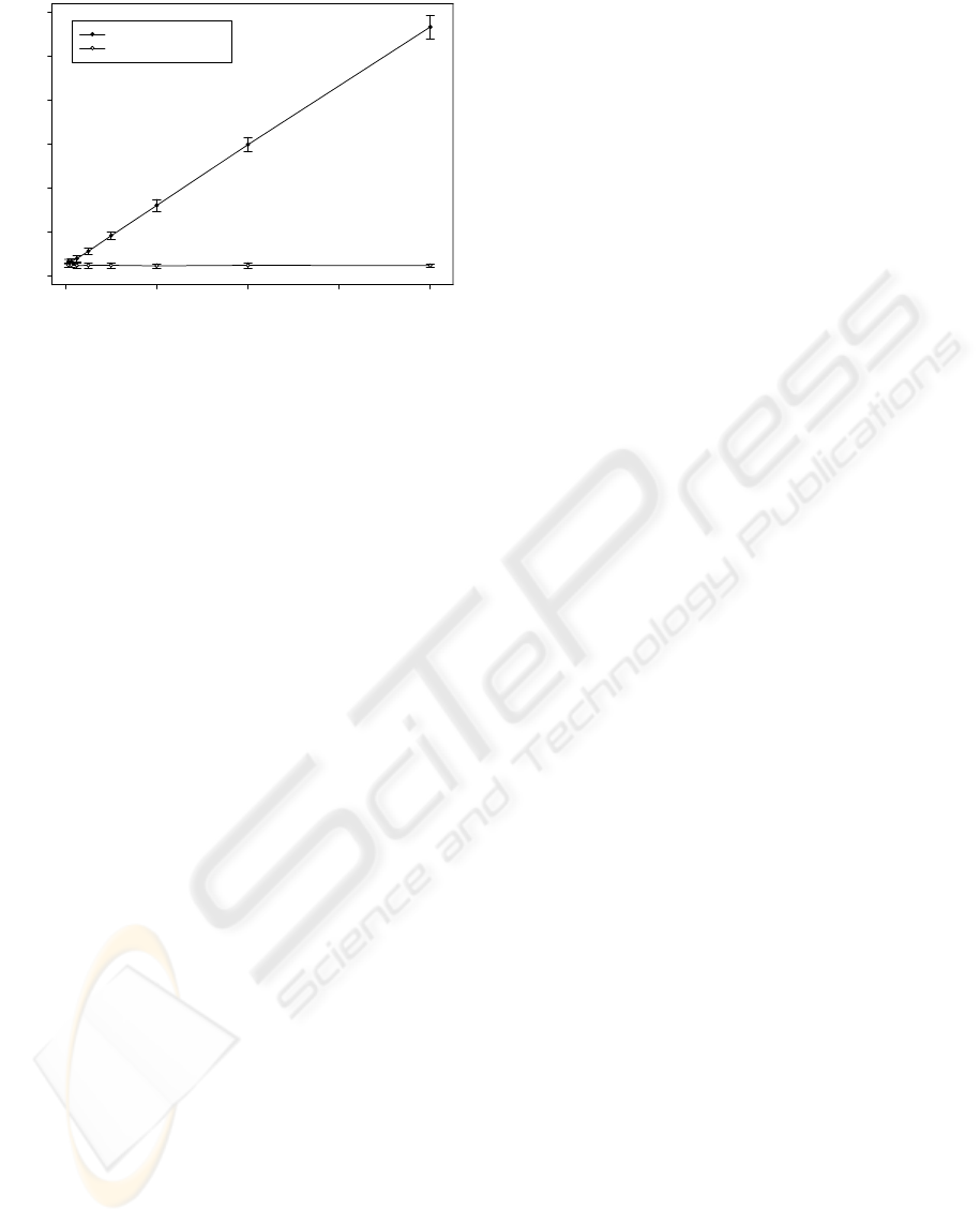
Frequency (Hz)
0 2000 4000 6000 8000
Time (ms)
0
50
100
150
200
250
300
All Fresnel zones
First Fresnel zone only
Figure 9: Results for the diffraction running time require-
ments simulation: average diffraction modeling running
time vs. frequency with error bars (standard deviation).
z beginning at position (85m, 75m, 75m) and end-
ing at position (85m, 85m, 85m)). The results of this
simulation are summarized in Figure 9 where the av-
erage running time and standard deviation for each
frequency band (obtained over 225 measurements) to
compute the diffraction modeling are given. When
considering the first Fresnel zone only, the difference
in running time from the smallest (11.42ms for the
200Hz center frequency) to the largest running time
(12.27ms for the 125Hz center frequency) is 0.85ms
and therefore, running time is approximately constant
across frequency. In contrast, the running time when
considering all Fresnel zones increases linearly with
frequency, ranging from 16.90ms (63Hz) to 283.42ms
(8000Hz). In addition to the first Fresnel zone only
implementation providing more accurate results (as
demonstrated in the simulation described in Section
4.1), its running time requirements are much less and
constant across frequency. This is of course directly
related to the additional time required to determine
the position of a secondary source in each additional
Fresnel zone in addition to calculating the visibility
weighting of each additional Fresnel zone relative to
the receiver.
5 CONCLUSIONS
This paper presented a simple method capable of
modeling acoustical edge diffraction effects in an effi-
cient manner. The method is inspired by the Huygens-
Fresnel principle which assumes a propagating wave-
front is composed of a number of secondary sources.
This fits nicely within particle-based (geometric)
acoustical modeling methods such as sonel map-
ping whereby acoustical wave propagation is approx-
imated by propagating sound particles (sonels) from
a sound source and tracing them through the environ-
ment. Experimental results demonstrate that diffrac-
tion effects can be approximated in a very simple and
efficient manner allowing computation at interactive
rates. Although the Huygens-Fresnel principle is a
rather simple approach, it can satisfactorily describe a
large number of diffraction configurations in an effi-
cient manner.
REFERENCES
Allen, J. B. and Berkley, D. A. (1979). Image method for
efficiently simulating small-room acoustics. Journal
of the Acoustical Society of America, 65(4):943–950.
Anonymous (2006). Sonel mapping: A stochastic acous-
tical modeling system. In Proc. IEEE International
Conference on Acoustics, Speech and Signal Process-
ing, Toulouse, France.
Calamia, P. T., Svensson, U. P., and Funkhouser, T. A.
(2005). Integration of edge-diffraction calculations
and geometrical-acoustics modeling. In Proceedings
of Forum Acusticum 2005, Budapest, Hungary.
Cremer, L. and M
¨
uller, H. A. (1978). Principles and Ap-
plications of Room Acoustics, volume 1. Applied Sci-
ence Publishers LTD., Barking, Essex, UK.
Funkhouser, T., Tsingos, N., Carlbom, I., Elko, G., Sondhi,
M., West, J. E., Pingali, G., Min, P., and Ngan, A.
(2004). A beam tracing method for interactive archi-
tectural acoustics. Journal of the Acoustical Society of
America, 115(2):739–756.
Hecht, E. (2002). Optics. Pearson Education Inc., San Fran-
cisco, CA. USA, 4 edition.
Jensen, H. W. (2001). Realistic Image Synthesis Using Pho-
ton Mapping. A. K. Peters, Natick, MA. USA.
Kapralos, B., Jenkin, M., and Milios, E. (2005). Acous-
tical modeling using a Russian roulette strategy. In
Proceedings of the 118
th
Convention of the Audio En-
gineering Society, Barcelona, Spain.
Keller, J. B. (1962). Geometrical theory of diffraction. Jour-
nal of the Optical Society of America, 52(2):116–130.
Krokstad, A., Strom, S., and Sorsdal, S. (1968). Calculat-
ing the acoustical room response by the use of a ray
tracing technique. Journal of Sound and Vibration,
8(1):118–125.
Kulowski, A. (1985). Algorithmic representation of the ray
tracing technique. Applied Acoustics, 18(6):449–469.
Tsingos, N., Carlbom, I., Elko, G., Funkhouser, T., and
Kubli, B. (2002). Validation of acoustical simulations
in the “Bell Labs Box”. IEEE Computer Graphics and
Applications, 22(4):28–37.
Tsingos, N. and Gascuel, J. (1998). Fast rendering of sound
occlusion and diffraction effects for virtual acoustic
environments. In Proc. 104
th
Convention of the Audio
Engineering Society, pages 1–14, Amsterdam, The
Netherlands.
GRAPP 2007 - International Conference on Computer Graphics Theory and Applications
248
