
PYRAMID FILTERS BASED ON BILINEAR INTERPOLATION
Martin Kraus
Computer Graphics and Visualization Group, Technische Universit
¨
at M
¨
unchen, Germany
Magnus Strengert
Visualization and Interactive Systems Group, Universit
¨
at Stuttgart, Germany
Keywords:
Signal processing, image processing, multi resolution, pyramid algorithm, graphics hardware.
Abstract:
The implementation of several pyramid methods on programmable graphics processing units (GPUs) in recent
years led to additional research interest in pyramid algorithms for real-time computer graphics. Of particular
interest are efficient analysis and synthesis filters based on hardware-supported bilinear texture interpolation
because they can be used as building blocks for many GPU-based pyramid methods. In this work, several new
and extremely efficient GPU-implementations of pyramid filters are presented for the first time. The discussion
employs a new notation, which was developed for the consistent and precise specification of these filters and
also allowed us to systematically explore appropriate filter designs. The presented filters cover analysis and
synthesis filters, (quasi-)interpolation and approximation, as well as discontinuous, continuous, and smooth
filters. Thus, a toolbox of filters and their efficient implementations for a great variety of GPU-based pyramid
methods is presented.
1 INTRODUCTION
Many techniques in real-time image processing em-
ploy the pyramid algorithm by Burt (Burt, 1981), and
GPU-based image processing is no exception to this
rule (Williams, 1983; Kr
¨
uger and Westermann, 2003;
Lefebvre et al., 2005; Strengert et al., 2006). Pyramid
methods are of particular interest because they usu-
ally feature a linear time complexity and require only
a limited number of switches of the render target.
Although modern GPUs offer an enormous ras-
terization performance, the actual rasterization budget
for each pixel often consists of the equivalent to only
a few dozens of texture reads. This is already a seri-
ous limitation for many image processing techniques,
which often employ large two-dimensional convolu-
tion filters. Thus, even GPU-based implementations
of complex image processing techniques are often re-
stricted to small image sizes and/or low frame rates.
Therefore, several very efficient techniques have been
developed to implement specific (often small) con-
volution filters on GPUs (Sigg and Hadwiger, 2005;
Green, 2005). Unfortunately, many of these tech-
niques are restricted to very specific filters and partic-
ular applications; thus, the efficient implementation of
many other filters is still a challenging task in GPU-
based image processing.
In this work, we generalize a recently published
technique (Strengert et al., 2006) for a 2×2 box anal-
ysis filter and a 2 × 2 B-spline synthesis filter. By
formalizing the underlying concept with the help of a
new notation, we are able to systematically explore
appropriate filter designs and present several filters
that can be more efficiently implemented on GPUs
using bilinear texture interpolation than previous pub-
lications suggested.
In order to make these filters and their imple-
mentations more easily accessible to readers who
are looking for particular filters, we have also in-
cluded some previously published filter implementa-
tions. Moreover, these filters should help to illustrate
our new notation and the systematic filter construction
suggested in this work. We classify filters as basic
filters presented in Section 3; i.e., convolution filters
without reduce or expand operation; analysis filters
presented in Section 4; i.e., convolution filters com-
bined with a reduce operation; and synthesis filters
presented in Section 5, which are combined with an
21
Kraus M. and Strengert M. (2007).
PYRAMID FILTERS BASED ON BILINEAR INTERPOLATION.
In Proceedings of the Second International Conference on Computer Graphics Theory and Applications - GM/R, pages 21-28
DOI: 10.5220/0002076300210028
Copyright
c
SciTePress
g
H0L
= h
synthesis
Ä
g
H1L
g
H1L
= h
analysis
Ä
¯
g
H0L
top of pyramid: g
H2L
(a)
image g
h
2´2
Ä g
filter h
2´2
S
(b)
h
2×2
⊗ g =
h
1,1
h
1,2
h
2,1
h
2,2
⊗
g
1,1
g
1,2
0
g
2,1
g
2,2
0
0 0 0
≡
0 0 0
0 h
1,1
h
1,2
0 h
2,1
h
2,2
⊗
g
1,1
g
1,2
0
g
2,1
g
2,2
0
0 0 0
=
h
1,1
g
1,1
h
1,2
g
1,1
+ h
1,1
g
1,2
h
1,2
g
1,2
h
2,1
g
1,1
+ h
1,1
g
2,1
h
2,2
g
1,1
+ h
2,1
g
1,2
+ h
1,2
g
2,1
+ h
1,1
g
2,2
h
2,2
g
1,2
+ h
1,2
g
2,2
h
2,1
g
2,1
h
2,2
g
2,1
+ h
2,1
g
2,2
h
2,2
g
2,2
(c)
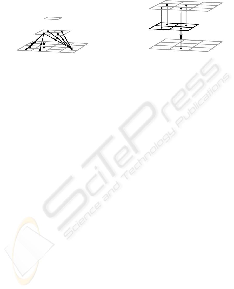
Figure 1: (a) An image pyramid consisting of 3 levels: g
(0)
, g
(1)
, and g
(2)
. (b) Illustration of the convolution of a 3× 3 image
g with a 2 × 2 filter h
2×2
. (c) The formal equation of the convolution illustrated in (b) including the equivalent 3× 3 filter
padded with zeros. Note the “mirrored” indices of h
2×2
and the “shift” of non-zero components in the resulting matrix.
expand operation. Analysis and synthesis filters are
further classified according to their featured smooth-
ness (in the limit of infinitely many reduce or expand
operations). Section 6 concludes this work with our
plans for future work.
2 PYRAMID METHODS ON GPUS
Pyramid methods usually convolve image data of one
pyramid level with a small analysis filter and reduce
the resulting image data to compute coarser pyramid
levels. This process is called analysis while the op-
posite process, called synthesis, expands image data
and convolves it with small synthesis filters to com-
pute finer pyramid levels; see Figure 1a. The reduce
and expand operation are also called downsampling
and upsampling, respectively.
Pyramid methods—more specifically spoken,
pyramid images—have been most successful in com-
puter graphics in the form of mipmap textures as
proposed by Williams (Williams, 1983). More re-
cently, the possibility to read pixel data of a raster-
ized image by texture interpolation without crucial
overhead led to new real-time image processing tech-
niques on GPUs (Green, 2005). For pyramid meth-
ods in GPU-based image processing, we suggested to
employ hardware-supported bilinear texture interpo-
lation for the reduce operation combined with a 2× 2
convolution filter (Strengert et al., 2006). However,
the only analysis filter presented in that work is a sim-
ple 2× 2 box filter. For the synthesis, we proposed to
employ bilinear texture interpolation for the combi-
nation of the expand operation and a 2× 2 synthesis
filter corresponding to the biquadratic B-spline sub-
division scheme (Catmull and Clark, 1978), which is
better known as the Doo-Sabin subdivision scheme
for regular quadrilaterals.
3 BASIC FILTERS
The filters discussed in this section are simple con-
volution filters without reduce or expand operation.
Thus, strictly speaking, they are not pyramid filters.
However, they act as building blocks for the more
complex filters discussed in Sections 4 and 5. A dis-
crete convolution of a filter mask h and an image g
resulting in an image f is denoted by
f = h⊗ g.
If the filter mask h is represented by an n
i
× n
j
matrix
and the image g is of dimensions n
r
× n
c
, the matrix
component f
r,c
for the row index r and the column
GRAPP 2007 - International Conference on Computer Graphics Theory and Applications
22

index c is defined by:
f
r,c
=
n
i
∑
i=1
n
j
∑
j=1
h
i, j
g
r−⌊i−n
i
/2⌋,c−⌊ j−n
j
/2⌋
.
Standard matrix notation is employed; i.e., row and
column indices are given in this order and indices start
with 1. Moreover, matrix products of column vectors
times row vectors (i.e., outer products of vectors) are
employed for separable filters.
Components of the image g with indices outside
the ranges from 1 to n
r
and 1 to n
c
, respectively, are
either set to 0 if the image g represents a filter mask,
or determined by clamping the indices to the valid
ranges. The dimensions of f depend on the partic-
ular application; in this work we usually determine
the dimensions of f by g’s dimensions; exceptions are
mentioned explicitly.
For even filter dimensions n
i
and n
j
, it is often
useful to think of the pixel positions of image f being
shifted by half a pixel along the diagonal relatively to
image g. In order to make this shift explicit, one can
use zero padding of the convolution mask; e.g., for
a 2× 2 convolution mask h
2×2
there is an equivalent
3×3 convolution mask with zeros in the first row and
column:
h
2×2
def
=
h
1,1
h
1,2
h
2,1
h
2,2
≡
0 0 0
0 h
1,1
h
1,2
0 h
2,1
h
2,2
.
For an illustration of these definitions and the de-
scribed shift of components of f , see Figures 1b and
1c.
As mentioned, g—and therefore f—may also rep-
resent filter masks. In this case, g and h denote two
convolution masks (applied from right to left), which
can be combined in one convolution mask f. In
fact, the main motivation for our formalism is to de-
compose complex filter masks (e.g., f ) into multiple
smaller filters (e.g., h and g, but usually more than
two), which are small enough (i.e., 2×2) to be imple-
mented by bilinear texture interpolations. In this way,
complex filters can be implemented by a sequence of
bilinear texture interpolations.
3.1 2× 2 Box Filter
The most important building block for the filters dis-
cussed in this work is the 2× 2 box filter, also known
as uniform, average, or mean filter:
h
2×2
box
def
=
1
4
1 1
1 1
.
Since this filter multiplies four neighboring pixels
with equal weights, it is easily implementable with
one hardware-accelerated bilinear texture image in-
terpolation. The sampling position for this texture in-
terpolation (usually specified by texture coordinates)
is determined by the position of the shared corner of
the four pixels (in the “little squares” model of pixels)
or the barycenter of the four pixels (if the pixels them-
selves represent sampling points in a uniform grid).
Due to our definition of the convolution, the sam-
pling point for the resulting matrix component with
indices r and c is located at the upper, left corner of
the pixel specified by r and c in the original source
matrix. (We assume a coordinate system that corre-
sponds to traditional matrix notation with the (posi-
tive) r axis pointing downwards and the (positive) c
axis pointing to the right.) This shift by half a di-
agonal of one pixel is more explicit in the equivalent
zero-padded 3 × 3 filter mask, which will be called
h
ց
box
:
h
2×2
box
≡ h
ց
box
def
=
1
4
0 0 0
0 1 1
0 1 1
.
The arrow in the symbol h
ց
box
indicates the position
of non-zero elements in the 3 × 3 matrix as well as
the shift of non-zero elements in the resulting matrix
illustrated in Figure 1c. Note, however, that the sam-
pling position for the bilinear texture interpolation is
shifted in the opposite direction relatively to the orig-
inal pixel position.
Obviously, there are further (non-equivalent) zero-
padded 3 × 3 filters, which shift pixel positions in
other directions; e.g., the opposite direction for the
filter h
տ
box
:
h
տ
box
def
=
1
4
1 1 0
1 1 0
0 0 0
.
This filter h
տ
box
can also be implemented by a bilin-
ear texture interpolation if the sampling point is set
to the opposite (lower, right) pixel corner. These two
box filters are the only building blocks for all filters
presented in this section and Section 4; i.e., all these
filters can be implemented by a decomposition into a
sequence of convolutions with h
ց
box
and h
տ
box
, and the
application of the corresponding sequence of bilinear
texture interpolations. The most basic example is the
3× 3 Bartlett filter discussed next.
3.2 3× 3 Bartlett Filter
Bartlett filters are also called triangular or (in partic-
ular in one dimension) triangle filters. They are sepa-
rable filters; therefore, they may be decomposed into
PYRAMID FILTERS BASED ON BILINEAR INTERPOLATION
23

matrix products of column times row vectors. In this
work, the 3× 3 Bartlett filter is of particular interest:
h
3×3
Bartlett
def
=
1
16
1 2 1
2 4 2
1 2 1
=
1
4
1
2
1
·
1
4
1 2 1
.
The separation into two one-dimensional filters
can also be expressed by a sequence of two convolu-
tions with these filters (with appropriate filter dimen-
sions and index mirroring). However, the represen-
tation as a convolution of box filters leads to a more
efficient implementation:
h
3×3
Bartlett
=
1
4
0 0 0
0 1 1
0 1 1
⊗
1
4
1 1 0
1 1 0
0 0 0
= h
ց
box
⊗ h
տ
box
= h
տ
box
⊗ h
ց
box
.
I.e., a sequence of two convolutions with h
ց
box
and h
տ
box
is equivalent to a single convolution with the 3 × 3
Bartlett filter h
3×3
Bartlett
. Therefore, the 3 × 3 Bartlett
filter may be implemented by a sequence of two bi-
linear texture interpolations corresponding to the two
2 × 2 box filters. Note that the second texture inter-
polation has to access the result of the first convo-
lution; thus, a hardware-accelerated implementation
will usually have to switch the render target in order
to access the previously rasterized image. Note also
that it is crucial to alternate between h
ց
box
and h
տ
box
;
otherwise, the discussed shifts would not cancel and
the resulting image would be shifted by one full pixel
position.
Since the 3×3 Bartlett filter h
3×3
Bartlett
is particularly
useful, we will also use it for building up more com-
plex filters. However, it is always understood that a
convolution with h
3×3
Bartlett
is equivalent to a sequence
of one convolution with h
ց
box
and one convolution with
h
տ
box
.
3.3 Gaussian Filters
Repeated convolutions of Bartlett filters are equiva-
lent to approximations of Gaussian filters if all non-
zero matrix components of the resulting filters are
considered; for example:
h
5×5
Gauss
def
=
1
16
2
1 4 6 4 1
4 16 24 16 4
6 24 36 24 6
4 16 24 16 4
1 4 6 4 1
≡ h
3×3
Bartlett
⊗ h
3×3
Bartlett
,
h
7×7
Gauss
def
=
1
16
3
1 6 15 20 15 6 1
6 36 90 120 90 36 6
15 90 225 300 225 90 15
20 120 300 400 300 120 20
15 90 225 300 225 90 15
6 36 90 120 90 36 6
1 6 15 20 15 6 1
≡ h
3×3
Bartlett
⊗ h
3×3
Bartlett
⊗ h
3×3
Bartlett
.
The basic reason for the approximation of Gaus-
sian filters is the central limit theorem; in fact, any
reasonable, positive filter will converge to a Gaussian
filter in the limit of infinitely many convolutions. In
the case of the box filter—and therefore also for the
Bartlett filter—the continuous convolutions are actu-
ally higher-order B-splines.
Since each convolution with a Bartlett filter can be
implemented by two bilinear texture interpolations,
n − 1 texture interpolations are necessary to imple-
ment an approximation to the convolution with an
n × n Gaussian filter. For comparison, a separable
n× n filter with fixed filter weights for the two one-
dimensional filters would require 2n nearest-neighbor
texture reads.
4 ANALYSIS FILTERS
Analysis filters are convolution filters that are com-
bined with a reduce operation, which reduces the
number of pixels by a factor of 2 in each dimen-
sion. Therefore, this operation is also called down-
sampling. In our notation it is indicated by a down-
ward pointing arrow:
f = h⊗
↓
g,
which defines the components of f as:
f
r,c
=
n
i
∑
i=1
n
j
∑
j=1
h
i, j
g
2r−⌊i−n
i
/2⌋,2c−⌊ j−n
j
/2⌋
.
The issue of shifts by half a pixel diagonal is dif-
ferent from the problem discussed in Section 3. Since
the number of components is divided by 2, it is prefer-
able to work with even dimensions of images and fil-
ter masks. Moreover, it is often preferable to use sym-
GRAPP 2007 - International Conference on Computer Graphics Theory and Applications
24
metric filter mask (in the sense of h
i
= h
n
i
−i+1
) in or-
der to avoid asymmetric weighting of even and odd
pixels.
For convenience we introduce a particular nota-
tion for the combination of an analysis filter with a
reduction by a factor of 2
m
in each dimension:
f = h⊗
m
↓
g,
which results in these components of f:
f
r,c
=
n
i
∑
i=1
n
j
∑
j=1
h
i, j
g
2
m
r−⌊i−n
i
/2⌋,2
m
c−⌊ j−n
j
/2⌋
.
Our notation combines a reduce operation with a
convolution in a single operation. Thus, if the con-
volution can be implemented with a bilinear texture
interpolation, the combination with the reduce opera-
tion is also implementable with a bilinear texture in-
terpolation. To this end, it is only necessary to use a
sparser grid of texture sampling points.
4.1 Discontinuous Filter
In order to illustrate our notation for analysis filters,
it is first applied to the 2 × 2 box filter, which is the
standard analysis filter for mipmap generation:
h
2×2
box
⊗
↓
g ≡ h
ց
box
⊗
↓
g.
In the case of analysis filters, the use of h
2×2
box
might be
preferable, although it is equivalent to h
ց
box
. One bilin-
ear texture interpolation is sufficient to implement this
analysis filter in pyramid methods (Strengert et al.,
2006).
The 2 × 2 box filter is classified as “discontinu-
ous” analysis filter because the equivalent filter for a
reduction of the dimensions by a factor of 2
m
is al-
ways a discontinuous box filter—even in the limit of
m → ∞: Consider the squared filter, which is defined
by a sequence of two reduce operations and convolu-
tions:
h
2×2
box
2
⊗
2
↓
g
def
= h
2×2
box
⊗
↓
h
2×2
box
⊗
↓
g
.
Thus, the actual (separable) box filter is:
h
2×2
box
2
=
1
4
0 0 0 1 1 1 1
⊤
·
·
1
4
0 0 0 1 1 1 1
.
For a general factor 2
m
, the equivalent filter
h
2×2
box
m
=
1
2
m
0. ..0
|
{z}
×(2
m
−1)
1. ..1
|
{z}
×2
m
⊤
·
1
2
m
0. ..0
|
{z}
×(2
m
−1)
1. ..1
|
{z}
×2
m
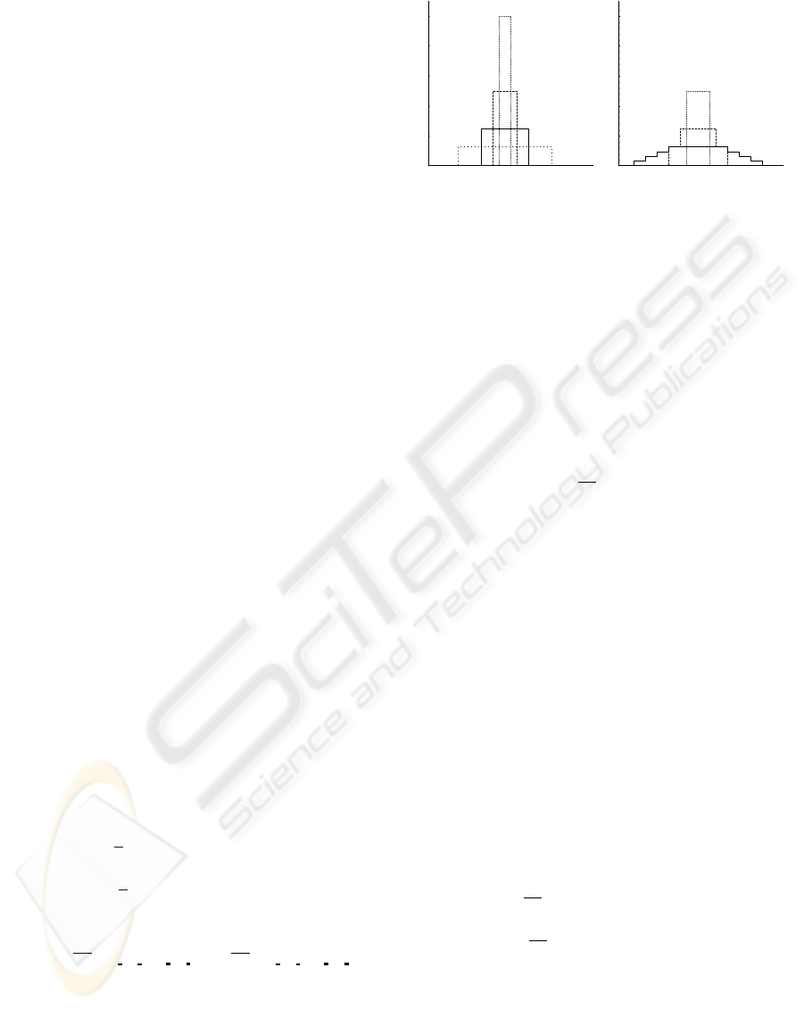
is still a discontinuous box filter. The one-
dimensional filter, which this separable filter is con-
structed from, is illustrated in Figure 2a for various
values of m. The same technique is employed to dis-
cuss and classify the smoothness of all analysis filters
presented in this section.
0.1
0.2
0.3
0.4
0.5
m = 1
m = 2
m = 3
m = 4
(a)
0.1
0.2
0.3
0.4
0.5
m = 1
m = 2
m = 3
(b)
Figure 2: (a) Powers of the 1D box filter mask correspond-
ing to h
2×2
box
. (b) Same as (a) for h
4×4
box
.
4.2 C
0
-Continuous Filter
While the 2 × 2 box filter is a discontinuous analysis
filter, the 4 × 4 box filter results in a C
0
-continuous
analysis filter in the limit of infinitely many analysis
steps. It is defined as:
h
4×4
box
def
=
1
16
1 1 1 1
1 1 1 1
1 1 1 1
1 1 1 1
,
h
4×4
box
⊗
↓
g ≡ h
ց
box
⊗
h
տ
box
⊗
↓
g
.
As indicated by our notation, this filter can be con-
structed by a reduce operation that includes a convo-
lution with h
տ
box
and a simple convolution with h
ց
box
.
Therefore, the implementation requires only two bi-
linear texture interpolations. However, there exists
one additional implementation difficulty: the first re-
duce operation will in general compute non-zero com-
ponents for the 0-th row and column. These interme-
diate results have to be stored and used in the second
convolution, otherwise the components of the first
row and column of the total result will be corrupted.
For the discussion of the smoothness of this anal-
ysis filter, we consider the equivalent (separable)
squared filter first:
h
4×4
box
2
=
1
16
0 0 0 0 1 1 2 2 2 2 2 2 1 1 0
⊤
·
·
1
16
0 0 0 0 1 1 2 2 2 2 2 2 1 1 0
.
The first three powers are illustrated in Figure 2b. In
contrast to the 2 × 2 box filter, the 4 × 4 box filter
has overlapping domains and therefore becomes C
0
-
continuous in the limit m → ∞; in fact, the 1D fil-
ter becomes piecewise-linear with a linear ascending
part, a constant part, and a linear descending part.
Our notation also suggests the construction of an
PYRAMID FILTERS BASED ON BILINEAR INTERPOLATION
25

(a) (b)
Figure 3: Pyramid image blurring using (a) the 2 × 2 box
analysis filter and (b) the 4 × 4 box analysis filter. (The
employed synthesis filter is discussed in Section 5.3.).
alternative combination of two box filters with one re-
duce operation:
h
3×3
Bartlett
⊗
↓
g ≡ h
ց
box
⊗
↓
h
տ
box
⊗ g
.
In the limit of m → ∞ this filter is also C
0
-continuous
(in fact, it is a triangle function); however, it includes
an additional undesirable shift and—what is worse—
the analysis of even and odd pixels becomes asym-
metric, which is likely to result in flickering artifacts
in animations. Therefore, the h
4×4
box
filter appears to be
the preferable C
0
-continuous analysis filter; e.g., for
pyramidal image blurring (Strengert et al., 2006) as
illustrated in Figure 3.
4.3 C
1
-Continuous Filter
By combining one reduce operation and three con-
volutions with box filters a C
1
-continuous filter can
be constructed, which we call h
4×4
quadratic
since it cor-
responds to a biquadratic B-spline in the limit of in-
finitely many analysis steps. The filter is defined as
h
4×4
quadratic
def
=
1
64
1 3 3 1
3 9 9 3
3 9 9 3
1 3 3 1
,
h
4×4
quadratic
⊗
↓
g ≡ h
ց
box
⊗
↓
h
3×3
Bartlett
⊗ g
.
The decomposition shows that three bilinear texture
interpolations are sufficient for an implementation of
this analysis filter.
The squared filter already indicates a shape similar
to the quadratic B-spline:
h
4×4
quadratic
2
=
1
64
0 0 0 0 1 3 6 10 12 12 10 6 3 1 0
⊤
·
·
1
64
0 0 0 0 1 3 6 10 12 12 10 6 3 1 0
.
In the limit of infinitely high powers it actually
converges to the C
1
-continuous biquadratic B-spline
function.
Another combination of three box filters and one
reduce operation is:
h
3×3
Bartlett
⊗
h
ց
box
⊗
↓
g
;
however, this analysis filter is only C
0
-continuous ac-
cording to our classification and requires one more
texture interpolation than h
4×4
box
. Yet another combina-
tion is:
h
տ
box
⊗
h
3×3
Bartlett
⊗
↓
g
,
which results in aC
1
-continuous analysis filter but in-
cludes an undesirable shift and an asymmetric weight-
ing of pixels. Thus, h
4×4
quadratic
is usually the preferable
C
1
-continuous analysis filter.
The construction of higher-order B-spline analysis
filters consists of additional convolutions with 2 × 2
box filters before the reduce operation is applied, e.g.:
h
5×5
cubic
⊗
↓
g ≡ h
ց
box
⊗
↓
h
3×3
Bartlett
⊗
h
ց
box
⊗ g
.
5 SYNTHESIS FILTERS
Analogously to analysis filters, synthesis filters are
convolution filters that are combined with an expand
operation, which increases the number of pixels by
a factor of 2 in each dimension. This operation is
also called upsampling and is indicated by a upwards
pointing arrow in our notation:
f = h⊗
↑
g,
where the components of f are:
f
r,c
=
n
i
∑
i=1
n
j
∑
j=1
h
r mod 2,c mod 2
i, j
× g
⌊(r+1)/2⌋−⌊i−n
i
/2⌋,⌊(c+1)/2⌋−⌊ j−n
j
/2⌋
.
The synthesis filters presented in this section
are strongly related to popular subdivision schemes,
which are very well known in computer graphics;
thus, we will considerably shorten the discussion by
refering the reader to the corresponding concepts for
subdivision schemes as discussed, for example, by
Zorin et al. (Zorin et al., 2000).
Similarly to the case of analysis filters, the com-
bination of an expand operation and convolution fil-
ters in our notation is closer to an efficient implemen-
tation using bilinear texture interpolation than tradi-
tional notations. One crucial difference to analysis
filters is the choice of sampling positions in the corre-
sponding bilinear texture interpolation. For most in-
terpolating synthesis filters, the sampling points are
GRAPP 2007 - International Conference on Computer Graphics Theory and Applications
26

the centers of pixels, their corners, and the midpoints
of their edges. This corresponds to face-split sub-
division schemes, which are also known as primal
schemes.
The most important alternative sampling posi-
tions are the positions of the Doo-Sabin subdivision
scheme for regular quadrilaterals (Strengert et al.,
2006). This alternative corresponds to vertex-split
subdivision schemes (also known as dual schemes)
and offers the advantage of symmetric computations
for all sampling positions while face-split schemes
distinguish between old and new positions.
In both cases, there are four different kinds of
sampling positions, which correspond to four convo-
lution filters h
1,1
, h
1,0
, h
0,1
, and h
0,0
with the super-
scripts determined by the new row index modulo 2
and the new column index modulo 2. This notation
is illustrated with the help of the well-known synthe-
sis filters for nearest-neighbor interpolation, bilinear
interpolation, and the biquadratic B-spline filter. On
the other hand, the suggested implementation of the
bicubic B-spline synthesis filter and the construction
of higher-order synthesis filters is a new result.
5.1 Discontinuous Filter
A discontinuous synthesis filter is already provided by
nearest-neighbor texture interpolation; thus, it is not
of particular interest for our work. However, we have
included it here for completeness and to demonstrate
our notation for this very basic synthesis filter:
h
1,1
nearest
def
= h
1,0
nearest
def
= h
0,1
nearest
def
= h
0,0
nearest
def
=
0 0 0
0 1 0
0 0 0
.
5.2 C
0
-Continuous Filter
Since bilinear texture interpolation already provides
a C
0
-continuous filter even without the overhead of
a pyramid method, the equivalent synthesis filter is
not very useful in itself; however, it may be used as a
building block for more complex synthesis filters. It is
called h
midpoint
because of the corresponding midpoint
subdivision scheme; its definition is:
h
1,1
midpoint
def
=
1
4
0 0 0
0 1 1
0 1 1
,
h
1,0
midpoint
def
=
1
2
0 0 0
0 1 0
0 1 0
,
h
0,1
midpoint
def
=
h
1,0
midpoint
⊤
,
h
0,0
midpoint
def
= h
0,0
nearest
.
Note that h
0,0
midpoint
corresponds to the convolution
filter for sampling positions at pixel centers while
h
1,1
midpoint
corresponds to the convolution filter for sam-
pling positions at their corners, and the remaining two
filters correspond to the centers of edges of pixels.
Also note that the first row and the first column of
the new image data will be sampled at the upper, left
corners of “old” pixels and the midpoints of edges be-
tween these positions. Therefore, the presented con-
volution filters will access “old” pixels of the 0-th row
and 0-th column. In practice, these lookups could re-
turn the corresponding pixel data of the first row and
first column, respectively. An alternative is to discard
the first row and first column of the resulting image.
5.3 C
1
-Continuous Filter
The synthesis filter discussed here corresponds to
the biquadratic B-spline subdivision scheme (Catmull
and Clark, 1978), also known as the Doo-Sabin sub-
division scheme for regular quadrilaterals or the two-
dimensional generalization of the Chaikin scheme. It
is an approximating vertex-split subdivision scheme;
thus, all pixels are processed in symmetric ways:
h
1,1
Doo-Sabin
def
=
1
16
0 0 0
0 9 3
0 3 1
,
h
1,0
Doo-Sabin
def
=
1
16
0 0 0
3 9 0
1 3 0
,
h
0,1
Doo-Sabin
def
=
h
1,0
Doo-Sabin
⊤
,
h
0,0
Doo-Sabin
def
=
1
16
1 3 0
3 9 0
0 0 0
.
The implementation of this synthesis filter
requires only one bilinear texture interpolation
(Strengert et al., 2006). Note that the convolution
for all boundary pixels of the resulting image accesses
pixels outside of the original image.
Our notation also suggests an equivalent but less
efficient implementation variant with two texture in-
terpolations instead of one:
h
Doo-Sabin
⊗
↑
g ≡ h
տ
box
⊗
h
midpoint
⊗
↑
g
.
Another synthesis filter may be constructed by re-
ordering the convolution filters:
h
midpoint
⊗
↑
h
տ
box
⊗ g
.
PYRAMID FILTERS BASED ON BILINEAR INTERPOLATION
27

Since the resulting synthesis filter is only C
0
-
continuous and requires one additional texture inter-
polation, there is no apparent advantage compared to
the C
1
-continuous h
Doo-Sabin
filter.
5.4 C
2
-Continuous Filter
The C
2
-continuous synthesis filter corresponding to
the bicubic B-spline subdivision scheme can be con-
structed easily in our notation with the help of one
additional convolution with a 2× 2 box filter:
h
cubic
⊗
↑
g ≡ h
ց
box
⊗
h
Doo-Sabin
⊗
↑
g
.
Permutations of the components of this construc-
tion result in less symmetric and/or less smooth syn-
thesis filters. On the other hand, the construction of
higher-order B-spline filters by additional convolu-
tions with 2 × 2 box filters should now be obvious.
Note, however, that h
ց
box
and h
տ
box
should appear in al-
ternating order as discussed in Section 3.
5.5 (Quasi-)Interpolating Filters
Unfortunately, the construction of aC
1
-continuous in-
terpolation synthesis filter is considerably more dif-
ficult than the approximation synthesis filter corre-
sponding to B-splines. If quasi-interpolation is suffi-
cient, the image data of the coarsest level can be con-
volved with a filter before the synthesis is performed.
The computation of appropriate convolution filters is
discussed by Litke et al. (Litke et al., 2001). For
example, a convolution filter for quasi-interpolation
with bicubic B-splines can be constructed that is im-
plementable with three texture interpolations:
1
24
−1 −2 −1
−2 36 −2
−1 −2 −1
≡
0 0 0
0
10
6
0
0 0 0
−
16
24
h
3×3
Bartlett
.
Our recommendation for an actually interpolat-
ing, C
1
-continuous synthesis filter corresponds to the
tensor-product generalization of the four-point sub-
division scheme. Since it is separable by construc-
tion, it can be implemented by a synthesis operation
for the rows followed by a synthesis operation for the
columns. This appears to result in the most efficient
implementation using 4.5 bilinear texture interpola-
tions per pixel of the resulting image.
6 CONCLUSION
In this work, a set of discrete pyramid filters that are
suitable for an efficient implementation based on bi-
linear texture interpolation has been presented. A
new, precise and consistent notation for convolutions
with these filters enabled us to construct appropriate
filters in a systematic way and helped us to discuss
many important implementation details. In particular,
we have proposed an efficient implementation of bi-
quadratic (and higher-order) B-spline analysis filters
and of bicubic (and higher-order) B-spline synthesis
filters.
Apart from applications of these filters, our plans
for future work on pyramid filters include more effi-
cient interpolating synthesis filters, three-dimensional
filters, and efficient implementations of derivative fil-
ters and nonlinear filters.
REFERENCES
Burt, P. J. (1981). Fast Filter Transforms for Image Pro-
cessing. Computer Graphics and Image Processing,
16:20–51.
Catmull, E. and Clark, J. (1978). Recursively Generated
B-Spline Surfaces on Arbitrary Topological Meshes.
Computer Aided Design, 10(6):350–355.
Green, S. (2005). Image Processing Tricks in OpenGL. Pre-
sentation at GDC 2005.
Kr
¨
uger, J. and Westermann, R. (2003). Linear Algebra Op-
erators for GPU Implementation of Numerical Algo-
rithms. ACM Transactions on Graphics, 22(3):908–
916.
Lefebvre, S., Hornus, S., and Neyret, F. (2005). Octree Tex-
tures on the GPU. In Pharr, M., editor, GPU Gems 2,
pages 595–613. Addison Wesley.
Litke, N., Levin, A., and Schroeder, P. (2001). Fitting Sub-
division Surfaces. In Proceedings IEEE Visualization
2001, pages 319–324.
Sigg, C. and Hadwiger, M. (2005). Fast Third-Order Tex-
ture Filtering. In Pharr, M., editor, GPU Gems 2,
pages 313–329. Addison Wesley.
Strengert, M., Kraus, M., and Ertl, T. (2006). Pyramid
Methods in GPU-Based Image Processing. In Pro-
ceedings Vision, Modeling, and Visualization 2006,
pages 169–176.
Williams, L. (1983). Pyramidal Parametrics. In Proceed-
ings ACM SIGGRAPH ’83, pages 1–11.
Zorin, D., Schr
¨
oder, P., DeRose, T., Kobbelt, L., Levin, A.,
and Sweldens, W. (2000). Subdivision for Modeling
and Animation. SIGGRAPH 2000 Course Notes.
GRAPP 2007 - International Conference on Computer Graphics Theory and Applications
28
