REAL-TIME RENDERING OF TIME-VARYING VOLUME DATA

USING A SINGLE COTS COMPUTER

Daisuke Nagayasu, Fumihiko Ino and Kenichi Hagihara

Graduate School of Information Science and Technology, Osaka University

1-3 Machikaneyama, Toyonaka, 560-8531 Osaka, Japan

Keywords:

Volume rendering, time-varying data, pipelined rendering, data compression, GPU, COTS.

Abstract:

This paper presents performance results of an out-of-core renderer, aiming at investigating the possibility

of real-time rendering of time-varying scalar volume data using a single commercial off-the-shelf (COTS)

computer. Our renderer is accelerated using software techniques such as data compression methods and thread-

based pipeline mechanisms. These techniques are efﬁciently implemented on a COTS computer that combines

multiple GPUs, CPUs, and storage devices using scalable link interface (SLI), multi-core, and redundant arrays

of inexpensive disks (RAID) technologies, respectively. We ﬁnd that the COTS-based out-of-core renderer

achieves a video rate of 35 frames per second (fps) for 258× 258× 208 voxel data with 99 time steps. It also

demonstrates an almost interactive rate of 4 fps for 512×512× 295 voxel data with 411 time steps.

1 INTRODUCTION

Volume rendering of time-varying data plays an in-

creasingly important role for understanding complex

time-varying phenomena in a wide range of ﬁelds

such as physical science and life science. This vi-

sualization technique produces animation sequences

that show how the three-dimensional (3-D) structure

evolves over time. Therefore, real-time rendering

with interactive rates is necessary to assist scientists

effectively in time-series analysis.

Due to the higher complexity of rendering

tasks, real-time rendering systems have traditionally

been implemented using high-performance comput-

ing (HPC) infrastructures such as supercomputersand

clusters of PCs. However, recent rapid advances in

graphics processing unit (GPU) technology (Mon-

trym and Moreton, 2005) have allowed us to use a

single commercial off-the-shelf (COTS) computer for

dealing with real-time rendering of non-time-varying

volume.

With respect to time-varying volume, on the other

hand, we further require a fast I/O mechanism to

achieve full performance on the GPU, because time-

varying data usually cannot be stored entirely in the

main memory. The lack of such an I/O mechanism

will result in poor performance, because the GPU usu-

ally waits for the data for the next time step.

To address this problem, prior systems (Lum et al.,

2002; Akiba et al., 2005; Strengert et al., 2005) re-

duced data size by data compression methods and

minimized I/O time using RAID technology (Patter-

son et al., 1988). Some HPC-based systems (Chiueh

and Ma, 1997; Bethel et al., 2000; Kniss et al., 2001;

Yu and Ma, 2005) also increased the throughput by a

pipeline mechanism that overlaps I/O operations with

computation.

Thus, many researchers have tried to achieve real-

time rendering of time-varying volume. However, it

is still not clear how well each technique contributes

to the acceleration. Furthermore, to the best of our

knowledge, most of the systems are implemented on

HPC systems. The objective of our project is to clar-

ify the contribution of each technique and to provide a

low-cost solution based on a single COTS computer.

In this paper, we present performance results of an

out-of-core renderer, aiming at investigating the pos-

sibility of real-time rendering of time-varying scalar

volume data using a single COTS computer. Our

renderer is accelerated using well-known techniques

such as data compression methods and thread-based

pipeline mechanisms. These techniques are efﬁ-

220

Nagayasu D., Ino F. and Hagihara K. (2007).

REAL-TIME RENDERING OF TIME-VARYING VOLUME DATA USING A SINGLE COTS COMPUTER.

In Proceedings of the Second International Conference on Computer Graphics Theory and Applications - GM/R, pages 220-227

DOI: 10.5220/0002076502200227

 SciTePress

ciently implemented on a COTS computer that com-

bines multiple GPUs, CPUs, and storage devices us-

ing scalable link interface (SLI) (nVIDIA Corpora-

tion, 2006), multi-core, and RAID technologies, re-

spectively. The key contribution of this paper is to

demonstrate that the techniques mentioned above are

necessary to achieve real-time out-of-core rendering

on a recent COTS computer.

The rest of the paper is organized as follows. Sec-

tion 2 presents a model that abstracts a COTS com-

puter. Section 3 describes our renderer with its un-

derlying acceleration techniques. Section 4 presents

performance results obtained on a COTS computer.

Section 5 concludes the paper.

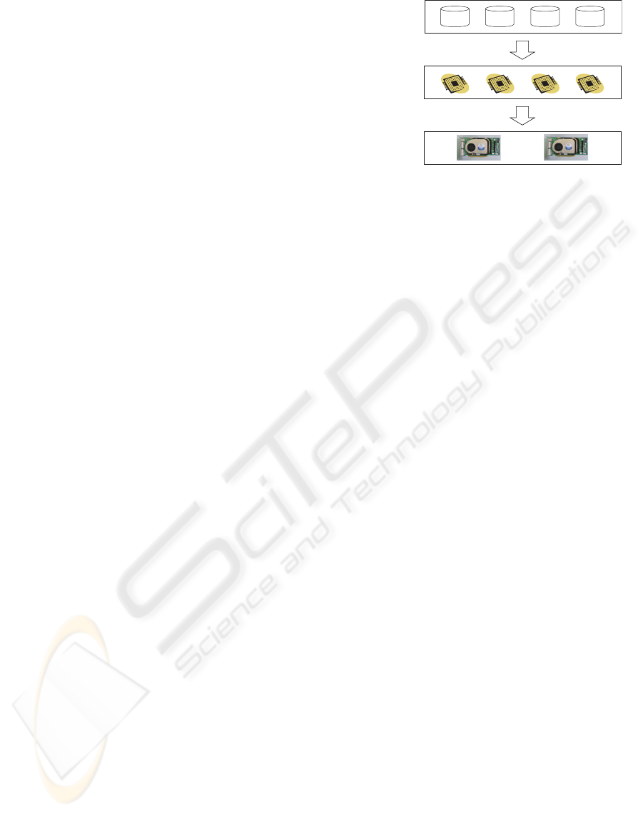
2 COTS COMPUTER MODEL

We ﬁrst present a COTS computer model to design an

efﬁcient real-time renderer on a COTS system. Fig-

ure 1 shows the model. We regard a COTS system

as a computer with hierarchical storages, having (1)

multiple disks, (2) main memory with multiple CPUs,

and (3) video memory with multiple GPUs. These hi-

erarchical storages are connected by two buses, each

with different bandwidths B

and B

, where B

and B

represent the bandwidth from disks to main memory

and that from main memory to video memory, respec-

tively. For example, our COTS system presented later

in Section 4 has B

= 103 and B

= 776 (MB/s).

Multiple disks can be realized using RAID tech-

nology (Patterson et al., 1988) at a low cost. We as-

sume that COTS systems have a RAID 0 array of disk

drives, where each disk drive separately stores differ-

ent parts of a ﬁle. This conﬁguration maximizes I/O

bandwidth, because different parts can be loaded si-

multaneously from different drives. However, I/O la-

tency is limited by the seek time of a single drive.

Therefore, data size should be large enough to make

the seek time relatively small over the entire I/O time.

Thus, RAID technology reduces I/O time by increas-

ing I/O bandwidth between storage devices and main

memory.

Similarly, multiplication of the remaining com-

ponents also can be realized by recent COTS tech-

nologies at a low cost. Multi-core and SLI technolo-

gies (nVIDIA Corporation, 2006) allow us to com-

bine multiple CPUs and GPUs into a single computer,

respectively. Note here that multiplication is done

also in a single GPU. That is, GPUs have multiple

shaders to exploit data parallelism in a rendering task

(Montrym and Moreton, 2005).

Thus, our COTS model multiplies key compo-

nents in a single computer. This multiplication

Main memory with

multiple CPUs by

multi-core technology

Video memory with

multiple GPUs by

SLI technology

Multiple disks by

RAID technology

Effective bandwidth

= 776 (MB/s)

Effective bandwidth

= 103 (MB/s)

Figure 1: COTS computer model with hierarchical storage

devices. This model assumes that the computer has multi-

ple disks, CPUs, and GPUs to exploit data-parallelism in an

out-of-core rendering task.

can be regarded as a low-cost parallel architecture,

as compared with HPC systems. From this view-

point, clusters of PCs are also a low-cost solution.

However, clusters are distributed-memory machines,

which require image compositing after parallel ren-

dering (Molnar et al., 1994). This involves high-

overhead communication at every frame, and more-

over, it takes longer time as the number of PCs in-

creases (Ma et al., 1994). Therefore, we think that

our COTS model is a reasonable solution in terms of

cost and parallelism.

3 COTS-BASED OUT-OF-CORE

RENDERER

In this section, we describe our renderer designed on

the basis of the COTS model presented in Section 2.

Figure 2 shows an overviewof our pipelined renderer.

3.1 Design Aspects

Since out-of-core rendering systems must stream data

through the two buses with different bandwidths B

and B

, we need some mechanisms to deal with this

bandwidth gap. Otherwise, the entire performance

will be limited by the slower bus, and thus, the GPU

and CPU might become idle during rendering.

The key idea to overcome this gap is to use a two-

stage compression method, which performs data de-

compression both on the CPU and the GPU. In this

method, the raw data must be converted into doubly-

compressed data in advance of rendering. During ren-

dering, the doubly-compressed data is decompressed

ﬁrstly by the CPU, and then by the GPU. This two-

stage method aims at hiding the gap by adjusting

data size to the bandwidth. Therefore, the maximum

performance will be achieved if the CPU generates

REAL-TIME RENDERING OF TIME-VARYING VOLUME DATA USING A SINGLE COTS COMPUTER

221

CPU side GPU side

Data loading

LZO decoding

Volume

rendering

Texture -based

rendering

PVTC decoding

(t+1)-th

data file

Data loading

LZO decoding

Volume

rendering

Texture -based

rendering

PVTC decoding

t-th

data file

SLI technology

Data loading

LZO decoding

Volume

rendering

Texture -based

rendering

PVTC decoding

Data loading

LZO decoding

Volume

rendering

Texture -based

rendering

PVTC decoding

Disk side

RAID

technology

I/O

thread

Decoding

thread

Rendering

thread

Multi-core technology

Time

step 3t

Time

step 3t+1

Time

step 3t+2

Time

step 3t+3

Time

step 3t+4

Time

step 3t+5

Figure 2: Overview of our pipelined rendering. The pipeline consists of three stages, each for data loading, LZO decoding,

and volume rendering. Doubly-compressed data is stored in disks as a ﬁle, containing successive volumes for three time steps.

times larger data as compared with the doubly-

compressed data loaded from disks.

We also use a pipeline mechanism to overlap I/O

operations with computation. This mechanism in-

creases the throughput of the renderer, because it al-

lows us to process successive data simultaneously at

different pipeline stages. In addition, the pipeline

mechanism contributes to hide the decompression

overheads incurred on the CPU.

Finally, once the time-varying data is sent to the

GPU, the ﬁnal image will be quickly generated by

the GPU. Our renderer uses a texture-based rendering

method (Cabral et al., 1994; Hadwiger et al., 2002),

which is fully accelerated by hardware components

in the GPU, such as texture mapping and alpha blend-

ing hardware. We currently use 3-D textures rather

than 2-D textures, because 2-D textures require three

times larger data (Hadwiger et al., 2002). Although

this might be a trivial problem for rendering of non-

time-varying data, it is critical for out-of-core (data-

intensive) rendering.

3.2 Two-Stage Data Compression

As shown in Figure 2, the two-stage compression

method performs data decompression both on the

CPU and the GPU. At the CPU side, we use

Lempel-Ziv-Oberhumer (LZO) compression (Ober-

humer, 2005). On the other hand, we use packed vol-

ume texture compression (PVTC) at the GPU side.

Thus, the raw data is ﬁrstly compressed by PVTC,

and then by LZO.

V3t+2(x,y,z)

V3t (x,y,z)

V3t+1(x,y,z)

Ct (x,y,z)

VTC

Each of 4x4x1 voxel (48-byte) blocks

are compressed into 8-byte data

R G B

3t 3t+1 3t+2

Block 1

R G B

3t 3t+1 3t+2

Block 2

...

A sequence of compressed blocks

each containing time-series data

Figure 3: Data compression using PVTC. Time-series

scalar voxels in the same location are packed into an RGB

voxel. This data packing generates a sequence of com-

pressed blocks, each containing time-series data.

This combination of different compression meth-

ods aims at taking architectural advantages of each

processing unit. As compared with the GPU, the

CPU has a memory hierarchy consisting of larger L1

and L2 cache and memory. These larger devices are

suited to LZO decompression, because it is based

on dictionary-based decoder (Ziv and Lempel, 1977),

which simply repeats data replication during decom-

pression.

In contrast, the GPU is based on a parallel ar-

chitecture capable of vector processing and single

instruction, multiple data (SIMD) processing (Mon-

trym and Moreton, 2005). This architecture exploits

higher parallelism than the CPU. Furthermore, some

GPUs have special hardware, such as a volume tex-

ture compression (VTC) decoder (OpenGL Extension

Registry, 2004), which provides us on-the-ﬂy decom-

pression of compressed texture. These architectural

advantages are fully utilized by PVTC, which is an

extension of VTC. As shown in Figure 3, the dif-

GRAPP 2007 - International Conference on Computer Graphics Theory and Applications

222

// Stage S1

Data loading(&ld->tstep);

Loading thread Decoding thread Rendering thread

/* Stage S2 */

LZO decoding(&dc->tstep);

// send a signal to the decoding thread

pthread_mutex_lock(&ld->mutex);

ld->tstep += 3; // update time step

pthread_cond_signal(&ld->ready);

pthread_mutex_unlock(&ld->mutex);

// send a signal to the rendering thread

pthread_mutex_lock(&dc->mutex);

dc->tstep += 3; // update time step

pthread_cond_signal(&dc->ready);

pthread_mutex_unlock(&dc->mutex);

// receive a signal from the loading thread

pthread_mutex_lock(&ld->mutex);

while (&ld->tstep <= &dc->tstep) {

pthread_cond_wait(&ld->ready,

&ld->mutex);

}

pthread_mutex_unlock(&ld->mutex);

// receive a signal from the decoding thread

pthread_mutex_lock(&dc->mutex);

while (&dc->tstep <= &rd->tstep) {

pthread_cond_wait(&dc->ready,

&dc->mutex);

}

pthread_mutex_unlock(&dc->mutex);

/* Stage S3(b) */

Texture-based rendering(&rd->tstep);

// send a signal to the loading thread

pthread_mutex_lock(&rd->mutex);

rd->tstep++; // update time step

pthread_cond_signal(&rd->ready);

pthread_mutex_unlock(&rd->mutex);

// Stage S3(a)

if (rd->tstep % 3 == 0) {

glCompressedTexImage3d(&rd->tstep);

}

glutPostRedisplay();

Idle callback functionDisplay callback function

// receive a signal from the rendering thread

pthread_mutex_lock(&rd->mutex);

while (&ld->tstep > &rd->tstep+lookahead) {

pthread_cond_wait(&rd->ready,

&rd->mutex);

}

pthread_mutex_unlock(&rd->mutex);

typedef struct stage_tag {

pthread_mutex_t mutex;

pthread_cond_t ready; // ready signal

int tstep; // time step

} stage_t;

stage_t *ld, *dc, *rd; // each for stage S1, S2, S3

const int lookahead = 7;

Va riables

Figure 4: Pseudocode of our thread-based pipeline mechanism. See text for details. Variable ‘lookahead’ limits the number

of stream data in the pipeline. This pipeline is allowed to process nine time steps of the data simultaneously, because each of

the three stages can have the data containing three time steps.

ference to VTC is that PVTC packs three successive

scalar volumes into an RGB-channel volume in ad-

vance of VTC. This data packing aims at exploiting

the temporal coherence in time-varying volume data.

The doubly-compressed data is obtained by the

following two steps (see also Figure 3).

1. PVTC compression. Three successive scalar vol-

umes are packed into R, G, and B channels of a

single volume, respectively. The packed data is

converted into a compressed texture by VTC. Re-

gardless of data contents, the compression ratio is

ﬁxed at a factor of 6, because VTC is a lossy com-

pression method.

2. LZO compression. The compressed texture is fur-

ther compressed by lossless LZO compression to

generate doubly-compressed data. The compres-

sion ratio achieved by LZO depends on the coher-

ence in the compressed texture.

In the rendering phase, the doubly-compressed

data is decoded by the following three stages.

S1. Data loading from disks. Doubly-compressed

data is loaded from disks to main memory. Note

here that a loaded ﬁle contains three successive

volumes due to PVTC data packing.

S2. LZO decoding on the CPU. The doubly-

compressed data is decompressed by LZO. A

compressed texture is then generated.

S3. Volume rendering on the GPU.

(a) Texture transfer. The compressedtexture is sent

from main memory to video memory.

(b) Texture-based rendering. Volumes stored in

R, G, and B channels of the compressed tex-

ture are rendered successively. Hardware-

accelerated on-the-ﬂy decompression is pro-

vided by the VTC decoder.

Note here that PVTC reduces not only data size

but also the number of data loads from disks, be-

cause it packs three volumes into a volume, namely

a ﬁle. Similarly, the number of data transfers from

main memory to video memory is also reduced to 1/3.

These reductions allow us to minimize overheads re-

quired for I/O operations and texture transfers.

3.3 Pipeline Mechanism

Our pipeline mechanism intends to increase the ren-

dering throughput by overlapping I/O operations with

computation, as shown in Figure 2. To realize this

mechanism by software, we use the POSIX thread

library (Nichols et al., 1996). Our renderer creates

three threads for each of stages S1, S2, and S3: the

loading thread, the decoding thread, and the render-

ing thread, as shown in Figure 4.

This mechanism is thread-safe if the following

conditions C1 and C2 are satisﬁed during execution.

REAL-TIME RENDERING OF TIME-VARYING VOLUME DATA USING A SINGLE COTS COMPUTER

223

Table 1: Storage devices used for experiments.

Component Speciﬁcation Latency (ms) B

: Bandwidth (MB/s)

Single disk 250GB SATA disk (Seagate Barracuda 7200.9) 13.8 57.0

RAID 0 Four 250GB SATA disks (Hitachi Deskstar T7K250) 12.8 103.3

Table 2: Datasets used for experiments.

Dataset

Volume size Time Raw ﬁle size per Compression ratio Coherence

(voxel) step time step (MB) PVTC PVTC+LZO Temporal Spatial

D1: Small jet 129× 129× 104 99 1.7 12.0 Low High

D2: Small vortex 128× 128× 128 99 2.0 6.5 Low Low

D3: Middle lung 256× 256 × 148 411 9.3

67.0 High High

D4: Middle jet 258× 258× 208 99 13.2 22.5 Low High

D5: Middle vortex 256× 256× 256 99 16.0 12.0 Low Low

D6: Large lung 512 × 512× 295 411 73.8 71.7 High High

C1. For all time steps t, the volume at time step t is

processed sequentially from stage S1 to stage S3.

C2. The rendering thread produces images in an as-

cending order of time step t.

To satisfy condition C1, we create threads

such that each of the threads is blocked with

pthread cond wait() until it receives a signal from the

upper thread. The upper thread, on the other hand,

sends a signal to the lower thread when it ﬁnishes the

responsible task. Also, the rendering thread sends a

wake-up signal to the loading thread after rendering.

Condition C2 can be satisﬁed by implementing a

ﬁrst-in, ﬁrst-out (FIFO) policy. To realize this, each

thread has variable ‘tstep,’ which stores the latest time

step processed at the corresponding stage. This infor-

mation is then used to prevent the stream data from

overtaking each other. That is, each thread is allowed

to process the t-th data if it is already processed by

the upper threads. Otherwise, it is repeatedly blocked

with pthread

cond wait() placed in a while loop.

4 EXPERIMENTAL RESULTS

We now show performance results of our renderer.

We implemented it using the C++ language, the

OpenGL library (Shreiner et al., 2003), the Cg toolkit

(Mark et al., 2003), and the POSIX threads library

(Nichols et al., 1996).

For experiments, we use a COTS computer

equipped with 2 GB of main memory and 1 TB of

Serial ATA disk devices shown in Table 1. The RAID

array is constructed using nVIDIA RAID, which is in-

cluded in nForce 590 SLI chipset. The computer has

a Pentium D (dual-core) CPU running at 3 GHz clock

speed and an nVIDIA GeForce 7900 GTX DDR SLI

card having 512 MB of video memory. The graph-

ics card is connected to a PCI Express 16X bus. The

effective bandwidth B

is 776 MB/s.

Table 2 summarizes six datasets D1–D6 used for

experiments. See also Figure 5 for their visualization

results. Datasets D1 and D2 (Ma, 2003) are ﬂuid dy-

namics datasets showing a turbulent jet and a turbu-

lent vortex ﬂow, respectively. Dataset D3 shows a

sequence of lung deformations representing a defor-

mation process of nonrigid registration (Hajnal et al.,

2001). The remaining datasets D4, D5, and D6 are

high-resolution versions of D1, D2, and D3, respec-

tively. Each dataset has voxels of 1-byte scalar data.

Datasets are rendered on a screen with an appro-

priate size: a 256 × 256 pixel screen for D1 and D2;

a 512 × 512 pixel screen for D3, D4, and D5; and a

1024× 1024 pixel screen for D6. The viewing direc-

tion is initially set to z-axis direction, and then it is

rotated 2 degrees around x- and y-axes when the time

step is updated.

4.1 Rendering Performance

To evaluate the performance gain of our renderer,

we compare it with 11 variations that utilize only a

part of the acceleration techniques: the RAID tech-

nology; the pipeline mechanism; and the two-stage

compression method. In the following, notations ‘R’

and ‘P’ indicates the RAID-equipped renderer and the

pipelined renderer, respectively. Notation ‘N’ repre-

sents the naive renderer without RAID and pipeline

mechanisms.

Figure 6 shows frame rates for 12 renderers. We

can see that the COTS-based out-of-core renderer

achieves a video rate of 35 frames per second (fps)

for 258× 258 × 208 voxel data with 99 time steps. It

also demonstrates an almost interactive rate of 4 fps

GRAPP 2007 - International Conference on Computer Graphics Theory and Applications

224

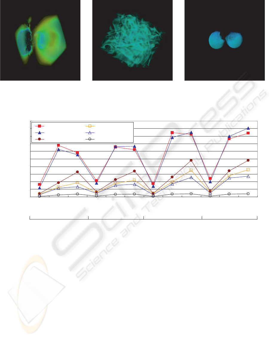
(a) (b) (c)

Figure 5: Produced images using three datasets. (a) D1: turbulent jet, (b) D2: turbulent vortex ﬂow, and (c) D3: deforming

lung.

100

D1: Small jet

D2: Small flow

D3: Middle lung

D4: Middle jet

D5: Middle flow

D6: Large lung

Rendering performance (fps)

Raw PVTC PVTC

+LZO

Raw PVTC PVTC

+LZO

Raw PVTC PVTC

+LZO

Raw PVTC PVTC

+LZO

R P RPN

Figure 6: Rendering performance in frames per second (fps). Notations ‘R’ and ‘P’ indicates the RAID-equipped renderer

and the pipelined renderer, respectively. Notation ‘N’ represents the naive renderer without RAID and pipeline mechanisms.

for 512 × 512× 295 voxel data with 411 time steps.

These performance results are competitive with prior

results (Akiba et al., 2005), which achieve 1.1 fps for

256× 256× 1024 voxel data with 400 time steps.

Improvement achieved by the pipeline mechanism

is not signiﬁcant if I/O time is not reduced by com-

pression or RAID. For example, the P renderer re-

sults in 1–17% improvement over the N renderer if

compression methods are not used. In contrast, com-

pression methods increase this improvement ratio to

3–91%. The RP renderer also increases the ratio to

49–73% by RAID. This means that most of the exe-

cution time is spent by I/O operations if we do not use

compression or RAID. Therefore, overlapping I/O op-

erations with other operations is not effective in this

case. Thus, we must reduce I/O time by RAID and/or

compression methods in order to maximize the per-

formance beneﬁts of the pipeline mechanism.

The improvement ratio of 3–91% also indicates

that two-stage compression is effective especially on

pipelined renderers. Such renderers allow us to over-

lap decompression overheads with I/O time, as we

mentioned in Section 3.1.

4.2 Breakdown Analysis

Table 3 shows the total executiontime T and its break-

down: T

, T

, and T

. T

and T

here represent the

time for data loading and LZO decompression, re-

spectively. T

is the time for texture-based rendering,

including the time T

for texture transfers.

Firstly, we analyze the effects of data compression

REAL-TIME RENDERING OF TIME-VARYING VOLUME DATA USING A SINGLE COTS COMPUTER

225

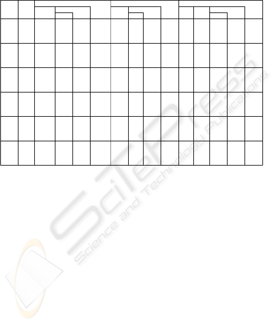
Table 3: Breakdown analysis of execution time. T represents the total execution time required for rendering of a volume at

a certain time step. Times T

, T

, and T

are the breakdown of time T, each representing the time for data loading, for LZO

decompression, and for texture-based rendering. T

includes time T

for texture transfers.

Data- Ren-

Raw PVTC PVTC+LZO

sets derer

I/O GPU I/O GPU I/O LZO GPU

T T

N 53.4 4.4 4.7 61.6 11.0 1.5 2.2 14.7 11.1 2.3 1.5 2.3 17.2

R 38.9 4.4 4.7 47.2 11.4 1.5 2.3 15.2 9.9 2.5 1.5 2.3 16.1

P 56.1 4.5 5.0 56.9 11.2 1.4 1.8 11.8 11.6 1.7 1.4 1.7 12.1

RP 40.5 4.6 5.2 41.3 12.5 1.4 1.8 13.1 11.4 1.7 1.4 1.7 11.9

N 75.8 4.0 4.9 82.5 11.5 1.8 2.6 15.9 11.4 2.3 1.8 2.8 18.0

R 48.0 3.9 4.9 54.6 10.6 1.9 2.8 15.0 8.5 2.5 1.8 2.9 15.0

P 69.5 3.6 4.2 70.4 12.2 1.7 2.1 12.8 11.1 2.0 1.7 2.1 11.8

RP 49.2 3.6 4.2 49.3 12.1 1.7 2.0 12.5 10.4 2.0 1.7 2.1 11.0

N 188.9 13.3 13.7 215.9 38.2 8.2 11.5 53.8 12.1 2.9 8.2 11.4 30.5

R 121.5 13.4 13.8 148.7 28.1 8.2 11.7 44.1 11.6 2.6 8.2 11.4 29.6

P 204.6 14.6 15.6 205.5 37.5 8.1 8.5 38.2 12.8 2.7 8.3 15.7 20.8

RP 128.3 14.1 15.0 129.1 28.3 8.1 8.7 29.1 11.8 2.8 8.0 15.3 20.7

N 231.1 19.0 19.4 264.2 54.8 11.7 16.4 75.6 23.2 9.6 11.7 16.3 53.6

R 142.8 19.0 19.4 175.6 35.3 11.8 16.4 56.1 16.0 8.8 11.8 17.1 45.1

P 229.9 23.0 23.9 230.8 49.8 11.6 12.2 50.4 20.4 9.6 11.9 20.3 28.6

RP 154.7 23.6 24.7 155.5 35.2 11.7 12.4 35.7 16.9 9.5 11.9 21.1 27.9

N 294.9 25.8 26.2 325.5 58.2 14.4 20.4 85.4 33.9 13.3 14.1 20.0 73.7

R 174.8 25.7 26.2 205.3 38.7 14.2 20.1 65.1 20.4 12.9 14.1 20.1 59.8

P 322.9 27.0 28.1 323.8 57.7 14.9 15.5 58.3 34.2 13.3 14.8 24.6 38.7

RP 193.3 31.7 32.7 194.0 38.7 14.9 21.7 40.1 22.7 13.6 15.1 28.1 36.9

N 1360.8 102.9 104.0 1482.5 207.2 65.1 125.6 366.9 26.6 19.7 121.2 183.0 261.9

R 766.0 102.8 103.9 895.3 137.4 67.5 127.0 299.9 19.6 19.4 126.3 187.9 260.2

P 1445.2 134.4 136.1 1446.1 209.7 93.6 196.0 270.7 27.0 20.7 91.9 216.4 253.6

RP 855.2 133.8 135.5 856.1 140.0 93.2 208.7 260.1 21.3 22.2 91.8 215.6 253.2

methods on the N renderer. In Table 3, we can see that

PVTC achieves 3.5–5.2 times higher performance, as

compared to the raw renderer. Furthermore, the com-

bination of PVTC and LZO achieves 1.2–1.8 times

higher performance than PVTC for datasets D3, D4,

D5, and D6. This performance gain is obtained by the

reduction of time T

. For D1 and D2, however, this

combination fails to show the performance gain over

PVTC. This is mainly due to the small ﬁle size. For

such small datasets, I/O time is mainly limited by I/O

latency, as we mentioned in Section 2. Therefore, the

renderer fails to reduce time T

, and moreover, it in-

creases time T

due to the decompression overheads.

Secondly, we compare the N renderer with the P

renderer to analyze the effects of the pipeline mech-

anism. In the N renderer, T

, T

, and T

accounts for

most of the entire time T. In contrast, the P renderer

overlaps these three overheads to reduce the entire

time T. As a result, it achieves a 1.9-fold speedup

over the N renderer at the best case. In many cases,

this pipeline mechanism reduces the entire time T

roughly to time T

, because the data loading stage is

the bottleneck stage in the pipeline. Therefore, the

decompression cost T

is usually hidden by time T

Thus, the pipeline mechanism is capable of hiding the

overheads of the two-stage compression method.

Finally, we compare the N renderer with the R ren-

derer to analyze the effects of RAID technology. This

technology reduces time T

by approximately 30%

for larger datasets. On the other hand, it fails to re-

duce time T

if it is approximately 10 ms. This re-

sult is reasonable because the threshold of 10 ms is

close to the I/O latency of a single disk shown in Ta-

ble 1. Thus, RAID technology is useful if the data

ﬁle is large enough to distribute it to every disk in the

RAID array.

5 CONCLUSION

We have presented performance results of an out-

of-core renderer for time-varying volume. Our ren-

derer is based on two software-based techniques

that increase the performance: (1) a two-stage data

compression method and (2) a thread-based pipeline

mechanism. The renderer is implemented efﬁciently

on a recent COTS computer equipped with multiple

GPUs, CPUs, and storage devices using SLI, multi-

core, and RAID technologies, respectively.

Experimental results indicate that the COTS-

GRAPP 2007 - International Conference on Computer Graphics Theory and Applications

226

based out-of-core renderer achieves a video rate of

35 frames per second (fps) for 258× 258× 208 voxel

data with 99 time steps. It also demonstrates an al-

most interactive rate of 4 fps for 512 × 512 × 295

voxel data with 411 time steps. These performance

results are competitive with prior results.

We also ﬁnd that most of the execution time is

spent by I/O operations if we do not use compres-

sion or RAID. Therefore, we think that I/O time

must be reduced by RAID and/or compression meth-

ods in order to maximize the performance beneﬁt of

the pipeline mechanism. The two stage compression

method achieves 3.6–7.1 times higher rendering per-

formance than the raw renderer. By integrating this

method into the pipeline mechanism, it achieves a

1.9-fold speedup at the best case. We think that the

pipeline mechanism is useful to hide the overheads of

data decompression.

One future work is to present performance com-

parison with traditional HPC-based renderers.

ACKNOWLEDGEMENTS

This work was partly supported by JSPS Grant-in-

Aid for Scientiﬁc Research for Scientiﬁc Research

(B)(2)(18300009) and on Priority Areas (17032007).

We would like to thank the anonymous reviewers for

their valuable comments.

REFERENCES

Akiba, H., Ma, K.-L., and Clyne, J. (2005). End-to-end data

reduction and hardware accelerated rendering tech-

niques for visualizing time-varying non-uniform grid

volume data. In Proc. 4th Int’l Workshop Volume

Graphics (VG’05), pages 31–39.

Bethel, W., Tierney, B., Lee, J., Gunter, D., and Lau, S.

(2000). Using high-speed WANs and network data

caches to enable remote and distributed visualization.

In Proc. High Performance Networking and Comput-

ing Conf. (SC’00), 23 pages (CD-ROM).

Cabral, B., Cam, N., and Foran, J. (1994). Accelerated vol-

ume rendering and tomographic reconstruction using

texture mapping hardware. In Proc. 4th Symp. Volume

Visualization (VVS’94), pages 91–98.

Chiueh, T. and Ma, K.-L. (1997). A parallel pipelined ren-

derer for time-varying volume data. In Proc. 2nd Int’l

Symp. Parallel Architectures, Algorithms and Net-

works (I-SPAN’97), pages 9–15.

Hadwiger, M., Kniss, J. M., Engel, K., and Rezk-Salama,

C. (2002). High-quality volume graphics on consumer

PC hardware. In SIGGRAPH 2002, Course Notes 42.

Hajnal, J. V., Hill, D. L., and Hawkes, D. J., editors (2001).

Medical Image Registration. CRC Press, Boca Raton,

FL.

Kniss, J., McCormick, P., McPherson, A., Ahrens, J.,

Painter, J., Keahey, A., and Hansen, C. (2001). Inter-

active texture-based volume rendering for large data

sets. IEEE Computer Graphics and Applications,

21(4):52–61.

Lum, E. B., Ma, K.-L., and Clyne, J. (2002). A hardware-

assisted scalable solution for interactive volume ren-

dering of time-varying data. IEEE Trans. Visualiza-

tion and Computer Graphics, 8(3):286–301.

Ma, K.-L. (2003). Time-Varying Volume Data Repository.

http://www.cs.ucdavis. edu/˜ ma/ITR/tvdr.html.

Ma, K.-L., Painter, J. S., Hansen, C. D., and Krogh, M. F.

(1994). Parallel volume rendering using binary-swap

compositing. IEEE Computer Graphics and Applica-

tions, 14(4):59–68.

Mark, W. R., Glanville, R. S., Akeley, K., and Kilgard,

M. J. (2003). Cg: A system for programming graphics

hardware in a C-like language. ACM Trans. Graphics,

22(3):896–897.

Molnar, S., Cox, M., Ellsworth, D., and Fuchs, H. (1994).

A sorting classiﬁcation of parallel rendering. IEEE

Computer Graphics and Applications, 14(4):23–32.

Montrym, J. and Moreton, H. (2005). The GeForce 6800.

IEEE Micro, 25(2):41–51.

Nichols, B., Buttlar, B., and Farrell, J. P. (1996). Pthreads

Programming. O’Reilly & Associates, Newton, MA.

nVIDIA Corporation (2006). nVIDIA SLI.

http://www.slizone.com/.

Oberhumer, M.F.X.J. (2005). LZO real-time data compres-

sion library. http://www.oberhumer.com/

opensource/lzo/.

OpenGL Extension Registry (2004). Gl

nv texture

compression vtc. http://oss.sgi.com/projects/ogl-

sample/registry/NV/texture compression %vtc.txt.

Patterson, D. A., Gibson, G. A., and Katz, R. H. (1988).

A case for redundant arrays of inexpensive disks

(RAID). In Proc. the ACM SIGMOD Int. Conf. Man-

agement of Data (SIGMOD ’88), pages 109–116.

Shreiner, D., Woo, M., Neider, J., and Davis, T. (2003).

OpenGL Programming Guide. Addison-Wesley,

Reading, MA, fourth edition.

Strengert, M., Magall´on, M., Weiskopf, D., Guthe, S.,

and Ertl, T. (2005). Large volume visualization of

compressed time-dependent datasets on GPU clusters.

Parallel Computing, 31(2):205–219.

Yu, H. and Ma, K.-L. (2005). A study of I/O methods

for parallel visualization of large-scale data. Parallel

Computing, 31(2):167–183.

Ziv, J. and Lempel, A. (1977). A universal algorithm for

sequential data compression. IEEE Trans. Information

Theory, 23(3):337–343.

REAL-TIME RENDERING OF TIME-VARYING VOLUME DATA USING A SINGLE COTS COMPUTER

227