FITTING 3D MORPHABLE MODELS USING IMPLICIT

REPRESENTATIONS

Curzio Basso and Alessandro Verri

DISI, Universit

a di Genova, Italy

Keywords:

3D Morphable Models, non-rigid registration, implicit surface representations.

Abstract:

We consider the problem of approximating the 3D scan of a real object through an afﬁne combination of

examples. Common approaches depend either on the explicit estimation of point-to-point correspondences

or on 2-dimensional projections of the target mesh; both present drawbacks. We follow an approach similar

to (Ilic and Fua, 2003) by representing the target via an implicit function, whose values at the vertices of

the approximation are used to deﬁne a robust cost function. The problem is approached in two steps, by

approximating ﬁrst a coarse implicit representation of the whole target, and then ﬁner, local ones; the local

approximations are then merged together with a Poisson-based method. We report the results of applying our

method on a subset of 3D scans from the Face Recognition Grand Challenge v.1.0.

1 INTRODUCTION

We consider the problem of approximating a target

3D surface with an afﬁne combination of (registered)

examples, under the assumption that both the exam-

ples and the target belong to the same object class.

When the assumption holds, the afﬁne space gener-

ated by the examples represents a model of the ob-

ject class, usually known as 3D Morphable Model in

case of faces (Blanz and Vetter, 1999). The model is

parameterized by the coefﬁcients of the afﬁne com-

bination. We consider the class of human faces; our

goal is to ﬁnd the best possible combination of the

available examples that approximates a given target.

This is essentially a problem of non-rigid registration,

where the available deformations are constrained by

the model; it can arise not only when building a 3D

Morphable Model (Allen et al., 2003; Basso and Vet-

ter, 2006), but also for performing 3D shape analysis

as done for images by (Blanz and Vetter, 2003).

In general, we might approach the problem in dif-

ferent ways, depending on the representation of the

target surface:

• the target is explicitly represented as a triangular

mesh, and the problem is solved in R

;

• the target is projected to R

, as depth map or

cylindrical projection;

• the target is represented implicitly in R

The ﬁrst strategy is essentially based on the Iter-

ated Closest-Point (ICP) registration algorithm (Besl

and McKay, 1992; Turk and Levoy, 1994). Although

originally used for rigid registration, it can be ex-

tended to non-rigid registration and to the case at

hand. This was demonstrated in (Allen et al., 2003),

where the possibility of using examples-based mod-

els was also mentioned. The drawback of this type of

approaches is the need of an explicit estimation of the

point-to-point correspondence between the model and

the target. Letting aside the problems due to holes in

the target, the search for corresponding points in R

might be computationally inefﬁcient.

The second approach, adopted by (Blanz and Vet-

ter, 1999) and (Basso and Vetter, 2006), avoids the

explicit estimation of point-to-point correspondences,

by minimizing the difference between the cylindrical

projections to R

of the target and the model. As well

as avoiding the direct search for corresponding points,

the projection to R

has the advantage of reducing the

problem dimensionality. However, this comes at the

cost of loosing some information about the 3D sur-

Basso C. and Verri A. (2007).

FITTING 3D MORPHABLE MODELS USING IMPLICIT REPRESENTATIONS.

In Proceedings of the Second International Conference on Computer Graphics Theory and Applications - GM/R, pages 45-52

DOI: 10.5220/0002077200450052

 SciTePress

faces, since the projection is not a parameterization of

the original surface. Moreover, the projection is usu-

ally non-linear and occlusions frequently occur.

In this paper we investigate the possibility of solv-

ing the problem representing the target implicitly in

. In doing so, we avoid the explicit correspondence

estimation, while still working in the original domain

of the data. Although it has never been applied to

our speciﬁc problem, (Ilic and Fua, 2003) have used

an implicit representation to reconstruct surfaces from

uncalibrated video sequences. In their work, how-

ever, it is not the target data that are represented im-

plicitly, but rather the model, a deformable template

that has to be matched to the data. Also related to

ours is the work of (Steinke et al., 2005), where the

problem of registering the target with a ﬁxed template

(not an example-based model) was solved represent-

ing both surfaces implicitly. The implicit represen-

tations where found using Support Vector Machines

(SVM).

Our work is based on a simpler implicit repre-

sentation of the target mesh, based on Radial Basis

Functions (RBF), while the model is still represented

explicitly. The implicit representation deﬁnes a sort

of potential ﬁeld in the space surrounding the target

surface, and can be used to deﬁne a robust cost func-

tion. In order to reduce the complexity of computing

the RBF for large meshes, we ﬁrst minimize the cost

function over a low resolution implicit representation,

and afterward we minimize it over higher resolution

patches of the target. Finally, the different patches are

blended together with a Poisson-editing approach (Yu

et al., 2004). In our work we assume that the target is

already coarsely aligned with the model.

2 BACKGROUND

In the following two subsection we brieﬂy expose

the basic notions our method builds upon: three-

dimensional Morphable Models, and implicit repre-

sentations of surfaces.

2.1 3D Morphable Models

A triangular mesh is deﬁned by a graph M = (V ,E);

V is a set of n vertices in R

and E is a set of edges

connecting the vertices. For convenience we write V

as a matrix

V = [v

.. .v

] =





.. . x

.. . y

.. . z





∈ R

3×n

. (1)

A set of m registered meshes, denoted by M

, will

share the same connectivity E but have different ver-

tices positions V

. We can naturally deﬁne the sub-

space of their afﬁne combinations, with coefﬁcients

a = (a

,. .., a

) ∈ R

, as

M(a) = (V (a), E), (2)

with

V (a) =

∑

i=1

and

∑

= 1. (3)

The afﬁne constraint is needed in order to avoid scal-

ing effects.

Note that rewriting eq. (3) in terms of the barycen-

ter

V =

∑

i=1

, (4)

we can eliminate the constraint on the sum of the co-

efﬁcients:

V (a) = V +

∑

i=1

−V ). (5)

Three-dimensional Morphable Models (3DMM) use a

representation for the afﬁne combination based on the

Principal Component Analysis (PCA) of the subspace

spanned by the V

−V . Without going into the details

of the PCA (Hastie et al., 2001, pp. 62-63), we only

report that for 3DMM eq. (5) is written as

V (α) = V +

m−1

∑

i=1

, (6)

where the U

are the principal components and the co-

efﬁcient vector a is replaced by α ∈ R

m−1

. See ﬁgure

1 for a simple two-dimensional example.

Assuming the examples are correctly registered,

any rigid transformation has been factored out from

the model. It can be explicitly included by deﬁning a

rotation matrix R and a translation vector t which are

applied to V (α):

V (α,ρ) = R(ρ) ·

(

V +

m−1

∑

i=1

)

+t(ρ) ⊗ 1

, (7)

where the last term is simply an n-times repetition of

the column vector t. R and t are parameterized by a

vector ρ ∈ R

, holding the coefﬁcients of the transfor-

mation (three for the rotation and three for the trans-

lation). Taking into account the rigid transformation,

the model is deﬁned by M(α,ρ) = (V (α,ρ),E).

2.2 Implicit Representations of 3D

Surfaces

An implicit representation of a given surface T ⊂ R

is a function F

: R

→ R such that the surface is one

GRAPP 2007 - International Conference on Computer Graphics Theory and Applications

of its level sets. That is, F

(v) = h for each v ∈ T , and

(v) 6= h otherwise, where h is a constant, typically

zero. Clearly, an example of implicit representation is

the Euclidean distance

(v) = min

w∈T

kv − wk. (8)

In order to deﬁne a cost function based on such

an implicit representation, we are interested in an an-

alytic form for the implicit function F

; we build it

following the lines of (Turk and O’Brien, 1999; Carr

et al., 2001). Given a certain 3D mesh, they look for

a function F(v) which is zero on the vertices and dif-

ferent from zero on a set of off-surface points. The

off-surface points are required to avoid the trivial so-

lution of a function identically zero over the whole

space. They are chosen to lie on the normal to the

surface at the mesh vertices. Let us denote by w

the

vertices and the off-surface points. Then, given a ra-

dial basis function φ(x), there exist a choice of scalar

weights d

and of a degree one polynomial P(v) such

that the function

F(v) =

∑

j=1

φ(v − w

) + P(v), (9)

satisﬁes the constraints F(w

) = h

and is also

smooth, in the sense that minimizes the energy

E =

Ω⊂R

+ F

+ 2F

, (10)

a generalization to R

of the thin-plate energy. In ﬁg-

ure 1 we show such an example of F

(v), where T is

a poly-line in 2D.

In practice, the unknown vectors d and p (coefﬁ-

cients of the polynomial) are the solutions of a linear

system. Given the matrices

Φ =







.. . φ







(11)

and

A =







1 x







(12)

one has to solve the system



Φ A









. (13)

Note that when the input mesh is large, the above

linear system, if dense, might become intractable. A

possible solution is to induce sparsity by choosing a

basis with compact support, but this on turn creates

extrapolation problems. In order to maintain spar-

sity and achieve good extrapolation behavior an op-

tion is to deﬁne multiple levels of resolution, as done

by (Ohtake et al., 2003). Without resorting to a com-

pact support basis, one can use Fast Multipole Meth-

ods to reduce both the storage and the computational

cost, as done in (Carr et al., 2001).

3 LOW RESOLUTION

APPROXIMATION

Given a 3DMM M(α,ρ) as deﬁned in section 2.1,

and a target mesh T , we formulate the approximation

problem as the optimization

,ρ

= argmin

α,ρ

D(M(α,ρ),T ), (14)

where D is a suitable function measuring the approx-

imation cost.

Assuming we have an implicit representation F

for the target mesh, we can deﬁne the cost of approx-

imating T by M(α,ρ) as

D(M(α,ρ),T ) =

∑

i=1

`(F

)), (15)

where the v

are the vertices of M(α,ρ), and ` might

be a quadratic loss or an M-estimator. The choice of

an M-estimator might be necessary when parts of the

model M are not present in the target T and inﬂuence

the correct approximation of the rest. Observe that

in the above deﬁnition we are essentially treating the

values F

) as residuals of the approximation. In

fact, if F

was the Euclidean distance function and

`(x) = x

, then D would correspond to an `

norm.

3.1 Optimization Scheme

In order to ﬁnd the minimum of the cost function (15),

we use a modiﬁed Newton’s method. For the sake

of clarity, in the following discussion we denote by

θ the vector of all model coefﬁcients, without distinc-

tions between α and ρ. Recall that the exact Newton’s

method consists in iteratively updating θ by adding

the solution p of the linear system

∇

D(θ) · p = −∇D(θ), (16)

where ∇

D(θ) denotes the Hessian matrix of D at θ.

The exact method converges to a minimum of D when

sufﬁciently close to it, but it does not in general; nev-

ertheless, there are a number of standard modiﬁca-

tions that make it more efﬁcient and robust. We em-

ploy a simple scheme, which keeps the Hessian ma-

trix sufﬁciently positive deﬁnite by adding a multiple

FITTING 3D MORPHABLE MODELS USING IMPLICIT REPRESENTATIONS

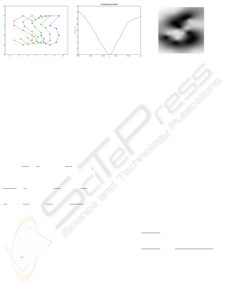
Figure 1: On the left, an example of a 2D morphable model M(α): two poly-lines, in red and blue, representing the characters

’S’ and ’3’. The green curves are linear combinations of the two examples, and can be written as the average shape plus a

deformation along the only principal direction. The amount of the deformation is given by the coefﬁcient α, whose values for

the three green curves are respectively α = {−0.5,0, 0.5}. If we consider the average shape (α = 0), it generates the implicit

representation on the right, where the gray-levels correspond to the values of F

(x), as deﬁned by eq. (9) with φ(x) = kxk.

The ﬁgure in the middle shows the corresponding cost function D(M(α),T ) as deﬁned by eq. (15) with `(x) = x

of the identity when required (Nocedal and Wright,

1999, Ch.6.3). Another modiﬁcation to the exact

method is that the update length is not unitary, but

it is determined by a backtracking procedure which

reduces the length if the update does not reduce D

(Nocedal and Wright, 1999, Ch.3.1).

Having the exact form of the implicit represen-

tation allows us to compute analytically the gradient

and the Hessian matrices of the cost function:

∂D

∂θ

∑

i=1



∇F

∂v

∂θ



, (17)

and

∂

∂θ

∑

i=1



∇F

∂v

∂θ



∇F

∂v

∂θ



∑

i=1



∂v

∂θ

· ∇

∂v

∂θ

+ ∇F

∂

∂θ



. (18)

In the above equations we used `

and `

to denote the

ﬁrst and second derivatives of the loss function com-

puted at F

); ∇F

and ∇

denotes the gradient

vector and the Hessian matrix of F

with respect to

the spatial coordinates, computed at v

In practice we choose ` to be the Tukey estimator,

that is

`(x) =

(

1 −



1 − (x/c)



if|x| ≤ c

/6 otherwise

(19)

with derivatives

(x) =

(



1 − (x/c)



if|x| ≤ c

0 otherwise

(20)

(x) =

(



1 − 5(x/c)



1 − (x/c)



if|x| ≤ c

0 otherwise

(21)

Note that the effectiveness of the Tukey estimator in

reducing the inﬂuence of model vertices not present

in the target depends on the scale of the constant c:

the smaller the constant, the smaller the inﬂuence of

missing vertices. On the other hand, small c’s require

a good pre-alignment of the model with the target. In

all our experiments we used c = 5.0.

The gradient and Hessian of F

depends on the

choice of the basis φ. Following (Carr et al., 2001), we

use the biharmonic basis function φ(x) = kxk, which

results in the smoothest solution to the interpolation

problem among all radial basis functions. Such a

function with non-compact support is also more suit-

able to inter- and extrapolation. The derivatives are

easily computed

∇φ(x) = x/φ, (22)

∇

φ(x) =



− ∇φ · ∇φ



/φ. (23)

Accordingly, we have

∇F

∑

j=1

− w

) + (p

, p

), (24)

∇

∑

j=1

− w



−

− w

)(v

− w

)

− w



(25)

3.2 Regularizing Prior

In many cases, in particular to avoid overﬁtting, it

might be convenient to add to the cost function (15) a

regularization term which penalizes excessively large

model coefﬁcients:

= D + η

E(α) + η

E(ρ), (26)

GRAPP 2007 - International Conference on Computer Graphics Theory and Applications

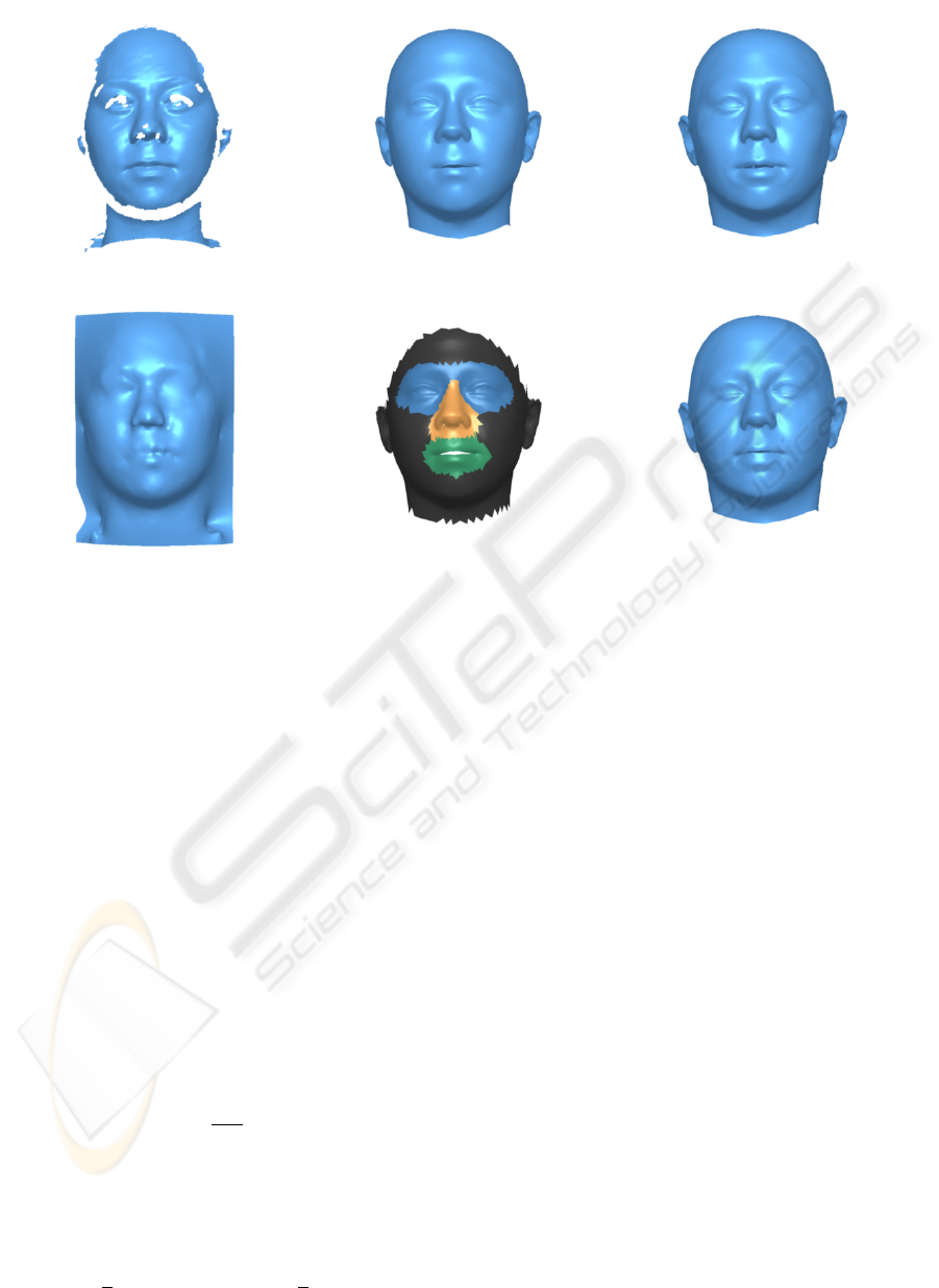
Figure 2: Examples of input data and the results of each approximation step. On the left column are shown the target (top

image) and the implicit representation of its subsampling (bottom). Fitting the model to the latter results in the shape in the

middle column, top image. The next step consist in separately ﬁtting the segments of the model, shown in the bottom-center

image, to corresponding parts of the target. The result is shown in the right column: on the top are the different approximations

stitched together, on the bottom the result of blending them.

where the parameters η

and η

weight the effect of

the regularization on the shape and the rigid parame-

ters, respectively.

A standard way to choose the regularization terms

consists in deriving them from prior probabilities. In

the case of the shape coefﬁcients, the PCA model

assumes for α a normal distribution with unit vari-

ance; for the rigid coefﬁcients we also assume a Gaus-

sian distribution with zero mean, but with empiri-

cally chosen variances. In both cases, we can deﬁne

a regularization term proportional to the inverse log-

likelihood. For a generic coefﬁcient θ with variance

we have

−log p(θ) =

2σ

+ const. (27)

so that we set (Σ

is the diagonal covariance matrix

for the rigid coefﬁcients)

E(α) =

kαk

and E(ρ) =

−1

ρ. (28)

4 SEGMENTED

APPROXIMATION

As noted in section 2.2, a direct solution of the inter-

polation problem by solving the linear system is com-

putationally and storage intensive. In fact, for high

resolution target meshes, the system is too large to be

allocated in memory. Rather than following one of

the methods mentioned in section 2.2, we decided to

overcome the problem by adopting a simpler multi-

resolution approach (refer to ﬁgure 2 for examples of

the intermediate steps outputs):

1. Coarse Approximation. We ﬁrst compute a

coarse approximation of the target. We select a

subset of the target mesh vertices, sampled with

probabilities proportional to the areas of the ad-

joining triangles, and use them as constraints of

the interpolation problem. The resulting implicit

surface is ﬁt with the procedure described in the

previous section.

2. Partitioning. Once we have obtained the coarse

approximation of the target, we can achieve a

higher resolution by repeating the process on

FITTING 3D MORPHABLE MODELS USING IMPLICIT REPRESENTATIONS

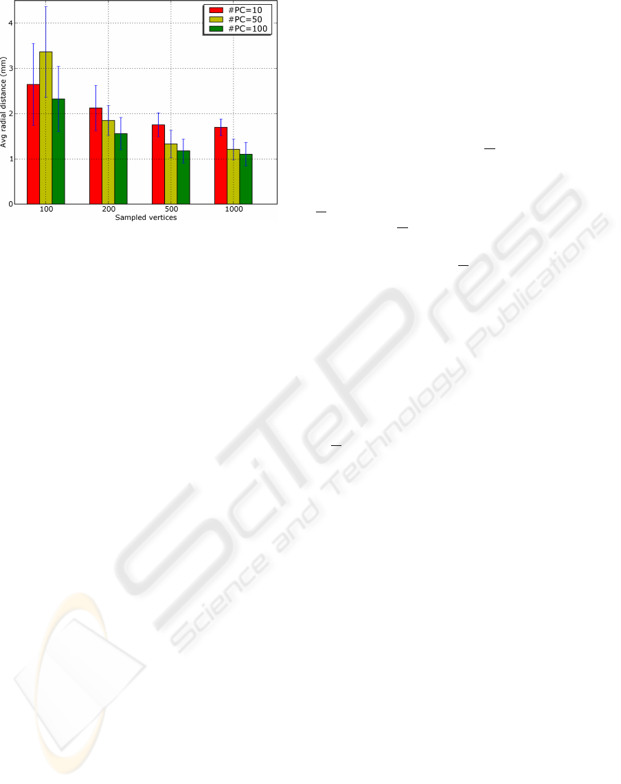
Figure 3: Dependency of the approximation on the number

of principal components used by the model and the number

of vertices sampled from the target surface.

smaller patches of the target and ﬁnally merging

the local approximations. To this aim, we manu-

ally deﬁned four regions on the model topology;

the regions are visible in ﬁgure 2, middle image

of the bottom row. Given the coarse approxima-

tion, we compute the bounding box of each re-

gion, we expand it in all directions by a ﬁxed

length (2 cm in our experiments), and select all the

target’s vertices falling inside the box. This results

in four overlapping subsets of the target vertices,

each one associated with a different segment of

the model.

3. Finer Approximations. For each subset of the

target vertices we build an (approximate) implicit

representation by sampling its vertices as done

in step 1. Although the subsets are again sub-

sampled, the ratio between the number of sampled

vertices and the total number of vertices clearly

increases, resulting in a more precise representa-

tion. The implicit surfaces are ﬁt again with the

usual procedure.

4.1 Blending

It is clear that the approximation method explained in

the previous section provides local results, which do

not match precisely at their boundaries. In order to

merge them smoothly, we use a variational approach

akin to the Poisson-based mesh editing of (Yu et al.,

2004), to which we refer for more details. The main

idea is to keep ﬁxed the positions of the vertices in the

interiors of the segments and let the other vertices re-

lax to the positions which minimize an elastic energy.

The procedure is as follows:

1. identify the boundaries of the patches;

2. for each vertex, compute its minimum distance

from the boundaries, by fast marching (Kimmel

and Sethian, 1998);

3. deﬁne the interior as the set of vertices with dis-

tance greater than a certain threshold (we used 0.5

cm);

Steps 1 to 3 deﬁne the mesh interior Ω and its com-

plement, the boundary region

Ω: an area with given

width that surrounds the segments boundaries. We

denote by ∂Ω the set of vertices in the interior Ω that

are connected to any vertex in the boundary region

Ω. While the vertices in Ω are ﬁxed, the positions of

the vertices in Ω are obtained by solving the Poisson

equation:

4. for all the vertices in Ω, ﬁnd their position solv-

ing a discretized Poisson equation using as bound-

ary conditions the positions of the vertices in ∂Ω

and as guidance ﬁeld the gradient of the coarse

approximation.

In practice, one solves the Poisson equation for the

ﬁeld of displacements from the coarse approximation

to the ﬁne one. This formulation yields a sparse linear

system of equations of the type ∆d

= 0, where ∆ is the

discrete Laplacian operator over the mesh (Taubin,

1995), and d

is the displacement of the i-th vertex

in Ω. The system is solved under the boundary con-

straints at ∂Ω, where the displacements are known.

5 RESULTS

The above method has been tested using as model a

sub-sampled version of the mixed expression-identity

3D Morphable Model built with the algorithm de-

scribed in (Basso and Vetter, 2006). The sub-

sampling is simple, since the reference template was

built by subdivision of a low-resolution one. Out of

around 40k vertices at full resolution, we retained ap-

proximately 2.5k. As well as reducing the number

of vertices, we also discarded the expression shape

components and all the texture components. The tar-

gets were a set of 165 range scans, randomly sampled

from the range data distributed for the Face Recog-

nition Grand Challenge v.1.0 (Phillips et al., 2005).

The scans were distributed with a list of landmark po-

sitions, which we used to pre-align the faces to the

model. The approximations have been performed us-

ing 99 model components and 500 sampled vertices

for building the implicit representations. We should

remark that these are preliminary experiments, and a

more in-depth study will follow.

GRAPP 2007 - International Conference on Computer Graphics Theory and Applications

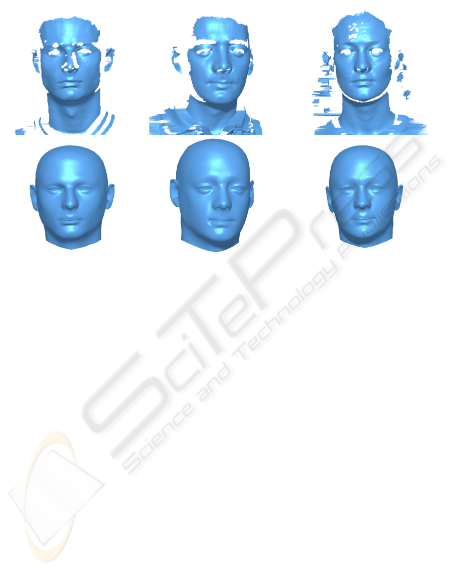
Figure 4: Some examples of approximations (bottom row, the original are on the top row). The average per-vertex radial

errors for the three examples are, respectively: 0.80, 0.86 and 0.80 mm.

We evaluated the goodness of the ﬁt by cylindri-

cally projecting the target and the approximation, and

computing the average absolute error (a radial dis-

tance) on the four segments. The rest of the head

model was not taken into account because of the hair

and clothes often present in the scans. Of the 165 re-

sults, we rejected three of them in which the error was

more than three standard deviations larger than the av-

erage. In the remaining 163 results, the average radial

error was 1.09 mm on the blended high-resolution re-

sult, with an average improvement with respect to the

low resolution approximation of 0.39 mm. Some of

the results are shown in ﬁgure 4.

We also ran a small experiment to assess the de-

pendency of the approximation on the number of prin-

cipal components used and the number of vertices

sampled from the target surface. We repeatedly com-

puted the low resolution approximations for a small

subset of test data (only four examples), varying the

two aforementioned parameters. The results are in

ﬁgure 3. The dependency on the number of principal

components used in the model behaves as expected:

up to a point, the more components are used the bet-

ter the approximation performance. This is not true

anymore when input is too noisy, as it probably oc-

curs when the number of sampled vertices is only 100.

More interestingly, the dependency on the number of

sampled vertices shows that an increase on the sample

rate pays off only up to a point, while the improve-

ment from 500 to 1000 is minimal.

6 CONCLUSION

We have presented a method which makes simple use

of the implicit representation of a surface to ﬁnd its

optimal approximation in terms of an afﬁne combi-

nation of examples. Implicit representations are ap-

pealing in general, because they are topology-free and

typically quite robust to holes in the data. In our

setting, they also offer the advantage of completely

avoiding the problem of estimating correspondences.

As we saw, however, the use of implicit rep-

resentations poses serious computational problems

when dealing with high-resolution meshes. There-

fore, we have proposed to tackle the problem in a

multi-resolution fashion, and we have shown how this

approach can provide good results without comput-

ing full-resolution representations. We should remark

that, in assessing the method, we considered its per-

formance only in absolute terms, without comparing

it with respect to other, already published algorithms.

FITTING 3D MORPHABLE MODELS USING IMPLICIT REPRESENTATIONS

This is certainly a deﬁciency of our work, and we

will have to correct it in the future. Nevertheless,

we believe that the absolute performance achieved by

our method on the Face Recognition Grand Challenge

range data is a strong indicator of its applicability to a

real-world scenario.

The sub-sampling of the original surface is further

motivated by the consideration that the model has also

a ﬁxed level of resolution. The resolution of the model

does not only dependent on the number of vertices of

its mesh, but especially on the number of training ex-

amples and of components used. It seems therefore

reasonable to tweak the resolution of the target so that

it matches the one of the model. On the other hand,

sub-sampling poses problems. This is particularly

clear when considering the approximation results ob-

tained on targets containing clothes or hairs. In the

best case these data are irrelevant, in the worst they

are harmful, since they will cause distortions in the

low-resolution implicit representation, which might

be enhanced by an unlucky sub-sampling. Prepro-

cessing of the targets which removes these data would

certainly improve the method’s performance and sta-

bility.

The future development will focus on two prob-

lems: ﬁrst, the choice of the optimal segments in

which the model is partitioned, and second, the in-

tegration of a texture model in the approximation

scheme.

ACKNOWLEDGEMENTS

This work has been partially supported by the FIRB

project RBIN04PARL.

REFERENCES

Allen, B., Curless, B., and Popovic, Z. (2003). The space

of human body shapes: reconstruction and parameter-

ization from range scans. In Proc. ACM SIGGRAPH

03.

Basso, C. and Vetter, T. (2006). Registration of expressions

data using a 3d morphable model. Journal of Multi-

media, 1(4):37–45.

Besl, P. and McKay, N. (1992). A method for registration

of 3-d shapes. IEEE Transactions on Pattern Analysis

and Machine Intelligence, 14(2):239–256.

Blanz, V. and Vetter, T. (1999). A morphable model for the

synthesis of 3d faces. In Proc. ACM SIGGRAPH 99,

pages 187–194. ACM Press.

Blanz, V. and Vetter, T. (2003). Face recognition based on

ﬁtting a 3d morphable model. IEEE Trans. Pattern

Anal. Mach. Intell., 25(9):1063–1074.

Carr, J. C., Beatson, R. K., Cherrie, J. B., Mitchell, T. J.,

Fright, W. R., McCallum, B. C., and Evans, T. R.

(2001). Reconstruction and representation of 3d ob-

jects with radial basis functions. In Proc. of ACM

SIGGRAPH 2001.

Hastie, T., Tibshirani, R., and Friedman, J. (2001). The

Elements of Statistical Learning. Springer Series in

Statistic. Springer.

Ilic, S. and Fua, P. (2003). Implicit meshes for modeling

and reconstruction. In Proc. Conf. Computer Vision

and Pattern Recognition 2003.

Kimmel, R. and Sethian, J. (1998). Computing geodesic

paths on manifolds. Proc. Natl. Acad. Sci. USA,

95(15):8431–8435.

Nocedal, J. and Wright, S. J. (1999). Numerical Opti-

mization. Springer Series in Operations Research.

Springer.

Ohtake, Y., Belyaev, A., and Seidel, H.-P. (2003). A

multi-scale approach to 3d scattered data interpola-

tion with compactly supported basis functions. In SMI

’03: Proceedings of the Shape Modeling International

2003, page 153, Washington, DC, USA. IEEE Com-

puter Society.

Phillips, P. J., Flynn, P. J., Scruggs, T., Bowyer, K. W.,

Chang, J., Hoffman, K., Marques, J., Min, J., and

Worek, W. (2005). Overview of the face recogni-

tion grand challenge. In Computer Vision and Pattern

Recognition (CVPR 2005), volume 1, pages 947–954,

Los Alamitos, CA, USA. IEEE Computer Society.

Steinke, F., Scholkopf, B., and Blanz, V. (2005). Support

vector machines for 3d shape processing. Computer

Graphics Forum, 24(3):285–294.

Taubin, G. (1995). A signal processing approach to fair

surface design. In SIGGRAPH ’95: Proceedings

of the 22nd annual conference on Computer graph-

ics and interactive techniques, pages 351–358, New

York, NY, USA. ACM Press.

Turk, G. and Levoy, M. (1994). Zippered polygon meshes

from range images. In SIGGRAPH ’94: Proceedings

of the 21st annual conference on Computer graph-

ics and interactive techniques, pages 311–318, New

York, NY, USA. ACM Press.

Turk, G. and O’Brien, J. F. (1999). Shape transformation

using variational implicit functions. In Proc. of ACM

SIGGRAPH 99.

Yu, Y., Zhou, K., Xu, D., Shi, X., Bao, H., Guo, B., and

Shum, H.-Y. (2004). Mesh editing with poisson-based

gradient ﬁeld manipulation. In Slothower, D., edi-

tor, Proc. ACM SIGGRAPH 04, pages 641–648. ACM

Press.

GRAPP 2007 - International Conference on Computer Graphics Theory and Applications