MULTI-MODE REPRESENTATION OF MOTION DATA

orn Kr

uger, Jochen Tautges and Andreas Weber

Institut f

ur Informatik II, Universit

at Bonn, R

omerstr. 164, 53117 Bonn, Germany

Keywords: Motion Capture, N -Mode SVD, Dynamic Time Warping, Motion Synthesis.

Abstract: We investigate the use of multi-linear models to represent human motion data. We show that naturally occur-

ring modes in several classes of motion can be used to efﬁciently represent the motions for various animation

tasks, such as dimensionality reduction or synthesis of new motions by morphing. We show that especially

for the approximations of motions by few components the reduction based on a multi-linear model can be

considerably better than one obtained by principal component analysis (PCA).

1 INTRODUCTION

The use and reuse of motion data recorded by mo-

tion capture systems is an important technique in

computer animation. Usually the motion data are

represented as sequences of poses, which in general

employ skeletal representations of motion data. In

the last few years also data bases of motions have

been used to synthesize or analyze motions in vari-

ous ways, see e.g. (Giese and Poggio, 2000; Troje,

2002; Kovar et al., 2002; Safonova et al., 2004; Kovar

and Gleicher, 2004; Ormoneit et al., 2005; Majkow-

ska et al., 2006).

Whereas the use of temporal alignments of mo-

tion in these data bases is well established (Bruderlin

and Williams, 1995; Giese and Poggio, 2000; Kovar

and Gleicher, 2003; Hsu et al., 2005) and the use of

linear models for representing motions and their di-

mensionality reduction by principal component anal-

ysis (PCA) is also a well established technique in var-

ious contexts (Barbi

c et al., 2004; Chai and Hodgins,

2005; Safonova et al., 2004; Glardon et al., 2004;

Troje, 2002; Ormoneit et al., 2005), little work has

been done to employ the multi-linear structure of the

motion data bases or to use the physics-based layer

for the temporal alignment. Whereas some work has

been done on using the physics-based layer (Majkow-

ska et al., 2006; Safonova and Hodgins, 2005) as dis-

tance measures, the only work we are aware of on

using multi-linear models for motion data is (Mukai

and Kuriyama, 2006).

The very successful use of multi-linear models in

the context of facial animation (Vlasic et al., 2005)

has been a major motivation for us to investigate them

in the context of motion capture data.

1.1 Our Contribution

In the following we will show that using naturally

occurring modes in several classes of motion can be

used to efﬁciently represent the motions in a multi-

linear model.

Using a data base of captured motions in which

several actors performed various motions in different

styles in different interpretations we build multi-mode

representations of various classes of motions:

• For one class of motions the motions have to be

time-aligned and warped.

Whereas in principal any time warping method

could be used for this task, we found it beneﬁcial

to use distance measures involving the physics-

based layer of a motion.

• A higher-order data tensor ∆ is built using differ-

ent modes of the motions.

• Using an higher-order SVD a core tensor Φ can

be computed, which can be used for representing

low-dimensional approximations of the motions.

We investigate the properties of the resulting

multi-mode representation, especially with respect to

Krüger B., Tautges J. and Weber A. (2007).

MULTI-MODE REPRESENTATION OF MOTION DATA.

In Proceedings of the Second International Conference on Computer Graphics Theory and Applications - AS/IE, pages 21-29

DOI: 10.5220/0002079200210029

 SciTePress

dimensionality reduction and its suitability for syn-

thesizing new motions by morphing.

We will show that especially for the approxima-

tions of motions by few components the reduction

based on a multi-linear model can be considerably

better than one obtained by principal component anal-

ysis (PCA).

2 MULTI-LINEAR ALGEBRA

For our tensor operations we use multi-linear algebra

which is an generalization of linear algebra.

A tensor is the basic mathematical object of multi-

linear algebra, it is a generalization of vectors (tensor

1st order) and matrices (tensor 2nd order). A tensor of

nth order can be thought as an n-dimensional block

of data. While within a matrix the two dimensions

(columns and rows) correspond to two modes, a ten-

sor can be build up with more general modes. A more

detailed description of multi-linear algebra is given in

(Vlasic et al., 2005).

2.1 Tensor Construction

There are different natural possibilities to ﬁll the data

tensor ∆ of our multi-mode model. Some do not re-

quire any preprocessing, some require e.g. a temporal

alignment of the motions. In the following we inves-

tigate the use of six different modes:

a) Actor Mode, all motions are captured from dif-

ferent people.

In our example motion data base, the actors were

given the same instructions how to perform the

motions. The ﬁve actors performing the motions

all have been healthy young adult male persons.

b) Style Mode, when possible we captured several

styles of the motion classes.

The meaning of style differs for the various mo-

tion classes; we describe them more closely in

section 4.

c) Repetition Mode (Interpretation Mode), all

motions are captured several times.

The instructors were told to stay within the same

verbal description of the motion and its style, but

nevertheless to have some variations in their inter-

pretations of the motion and the style.

These are quite generally applicable modes, they con-

sist of complete motions that span the space of the

considered motion classes.

The following modes are of a more technical na-

ture.

d) Data Mode, all information of a motion is stacked

into a single vector.

e) Frame Mode, this mode space is spanned by the

frames of the captured motions.

f) DOF Mode, all motion degrees of freedom are

separated in this mode. This mode depends on the

representation of the motion data.

They give a description of how the motion data are

arranged for the tensor construction. Either we stack

a complete motion into the Data Mode or the motion

is split into the Frame and DOF Mode. In (Mukai

and Kuriyama, 2006) the authors only focus on joint,

time and motion correlations, hence they are just us-

ing some technical modes.

2.2 Data Tensor

A tensor with the smallest number of modes was cre-

ated by using the natural modes a, b and c. Therefore

the motion data have to be ﬁlled into one vector to

construct the data mode. The matrix of size n × f,

which represents one motion, is stacked into one col-

umn. With this arrangement we obtain a tensor in the

size of f · n × a × b × c, where a is the number of ac-

tors in the Personal Mode, b is the size of the different

motion styles used for the Style Mode, c is the num-

ber of motion sequences in the Repetition Mode, f is

the number of frames in the Frame Mode and n is the

number of degrees of freedom for the given motion

representation.

A further tensor of a higher order is constructed

by using the three natural modes and the Frame and

DOF Mode. The result is a data tensor ∆ which has a

size of f × n × a × b × c.

2.3 N -Mode SVD

Similar to (Vlasic et al., 2005), the data tensors ∆

can

be transformed by an N -mode singular value decom-

position (N -mode SVD). For this purpose we used the

N-way Toolbox (C. A. Andersson and R. Bro, 2000).

The result is a tensor Φ

and respective matrices U

Mathematically this can be expressed in the following

way:

∆

= Φ

i,1

i,2

. . . ×

i,n

Where ×

describes the mode-n product. Mode-n-

multiplying a tensor T with matrix M replaces every

mode-n-vector v of T with a transformed vector M v.

A reduced model Φ

can be obtained by truncation

of insigniﬁcant components from Φ

and of matrices

, respectively. In the special case of a 2-mode ten-

sor this procedure is equivalent to principal compo-

nent analysis (PCA).

GRAPP 2007 - International Conference on Computer Graphics Theory and Applications

2.4 Motion Reconstruction

Once we have obtained the reduced model Φ

and

its associated matrices U

, we are able to approx-

imate any original motion. This is done by ﬁrst

mode-multiplying the core tensor with every matrix

belonging to a technical mode, and then mode-

multiplying the resulting tensor with one row of every

matrix belonging to a natural mode.

Furthermore, with this model in hand, we can gen-

erate an arbitrary interpolation of original motions by

using linear combinations of rows of U

with respect

to the natural modes.

3 TIME WARPING

Dynamic time warping (DTW) algorithms are widely

used in motion data processing to get a temporal

correspondence of the used motions. Such a corre-

spondence is needed to get reasonable realistic results

when synthesizing motions (Bruderlin and Williams,

1995; Giese and Poggio, 2000; Kovar and Gleicher,

2003). The result of a time warp depends on the used

algorithm, the given distance measurement and the

features with which the motions are compared. Until

now mainly kinematic features were used to compare

whole body motions. Dynamic features were only

used in the context of spliced body motions (Majkow-

ska et al., 2006).

3.1 Iterative Multi-scale Dynamic Time

Warping

We use the Iterative Multi-scale Dynamic Time Warp-

ing (IMDTW) algorithm presented by (Zinke and

Mayer, 2006). This enhanced algorithm is used be-

cause it has no quadratic runtime and does not need

quadratic memory space. This goal is reached by

combining two approaches:

• The possible pathes are restricted

• The path is searched iteratively with several reso-

lutions of the cost matrix

This iterative dynamic time warping algorithm works

on windows of the given (maybe high dimensional)

time series. After the ﬁrst iteration we have got a path

through the low resolution DTW matrix. We use a

tube around this path for the next iteration where we

calculate this tube with a smaller windows size what

results in a higher resolution.

3.2 Distance Measure

Our time warping algorithm is parameterized with the

following distance measure. For every frame i of a

considered motion we build a frame feature vector

f(i). This vector contains all properties of the mo-

tion that should be used for comparison. These frame

feature vectors are put together over a frame window

f(i), . . . , f(i + n) as normalized sum to compute a

feature vector F(i). Now we use the scalar product

of these feature vectors to compute a distance between

two motions:

D(F

(i), F

(j)) = 1 − hF

(i), F

(j)i

By this method we can handle a lot of different

features parallel. It is also possible to give a speciﬁc

feature a special weight by scaling. This feature then

contributes more to the direction the vector points in.

3.3 Distance Features

We found it very beneﬁcial to include features on the

physics-based level. For this purpose the mass from

all segments of a skeleton and their center of mass

have to be calculated. We use the heuristics based on

anthropometric tables described in (Robbins and Wu,

2003) for this purpose.

In addition to the center of mass (and its acceler-

ation) of the entire body we also use the angular mo-

mentum of the body segments as physics-based fea-

tures for comparing motions. Using a local coordi-

nate system aligned to the motion, these features are

independent of the starting position and orientation of

the root segment. Although this local coordinate sys-

tem strictly speaking is not an inertial system the oc-

curring pseudo-forces are rather negligible for typical

human motions.

All these simple features give a lot of information

on the viewed motions. Based on the acceleration of

the center of mass it is, for example, simple to de-

tect non-contact phases. Then the COM-acceleration

is equivalent to acceleration due to gravity when the

body has no ground contact:

COM

≈ a

earth





0.0

−9.81

0.0





Figure 1 shows the acceleration of the center of

mass of a dancing motion. There are three non-

contact phases that can be easily detected by analyz-

ing the y-component.

Figure 2 shows two distance matrices produced

by our DTW algorithm when comparing two walk-

ing motions. In dark areas the motions are equal, in

MULTI-MODE REPRESENTATION OF MOTION DATA

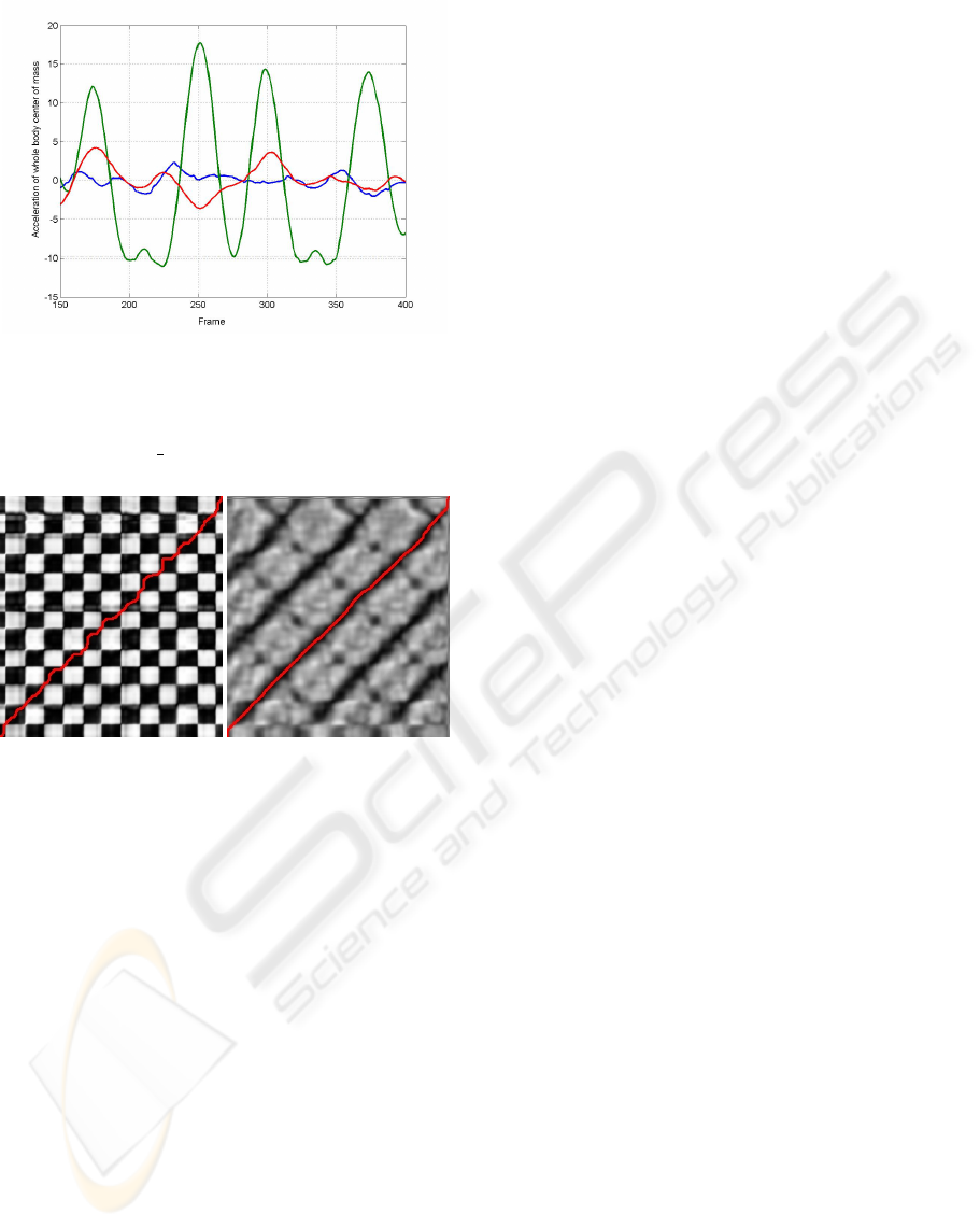
Figure 1: Accelerations of the center of mass of the entire

body of a dancing motion involving different jumps. One

can see two long non-contact phases corresponding to two

long jumps and one short intermediate non-contact step (ex-

tract from motion 05 16 from CMU mocap data base.)

Figure 2: DTW distance matrices calculated on the base of

different features. Acceleration of the whole body center of

mass (left), acceleration of the whole body center of mass,

hands and feet (right). The best warping paths are drawn

red.

brighter areas the motions are unequal, correspond-

ing to the given features. The red line is the warping

path found by the algorithm. The left one is based

only on the acceleration of the center of mass. In this

checkerboard-like pattern we have thirteen black di-

agonals. This shows that we can not differentiate be-

tween the steps. If we add the acceleration of the feet

to our features, the result gets obviously better. This

can be seen in the right picture of ﬁgure 2. There we

have got ﬁve dark diagonals, so steps made with the

same foot are detected as similar.

The right matrix is not as symmetric as the left

one. This shows that the motion is not similar to the

same backward motion.

Depending on the motions that should be time

warped, one can select speciﬁc features.

For walking motions the movement of the legs

gives the most important features, if the steps should

be synchronized. For Karate-like kicking motions

the foot that makes the kick is most important. The

moments, in the compared motions, where the leg is

stretched have to be matched to each other. There-

fore features from this leg should get a higher weight.

Another example we tested are cartwheel motions. To

get a good correspondence for these motions, features

that describe the motion of hands an feet are useful. A

result of this warping technique for a walking motion

is presented in the video.

4 RESULTS

For our experiments we built our motion model

for three motion classes: walking, grabbing and

cartwheel motions. For all of these motion classes

we constructed data tensors with motion representa-

tion based on Euler angles and based on quaternions.

Initially some preprocessing was required, consisting

mainly of the following steps. All motions were

a) ﬁltered in the quaternion domain with a smooth-

ing ﬁlter described in (Lee and Shin, 2002);

b) aligned over time by the time warping using

physics-based distance features;

c) moved to the origin with their root node and ori-

ented to the same direction;

d) ﬁnally sampled down to a frame-rate of 30 Hz.

By applying the N-Mode SVD on the data tensors

that were constructed of these motions we got the

core-tensors Φ that were used for the following ex-

periments.

4.1 Walking Motions

For this motion class we used walking motions out

of our database, from ﬁve actors which were asked to

perform the following four motions for three times:

• walk four steps in a straight line.

• walk four steps in a half circle to the left side.

• walk four steps in a half circle to the right side.

• walk four steps on the place.

All motions had to start with the right foot. All mo-

tions were aligned over time to the length of the ﬁrst

motion of actor one. The ﬁve actors performing the

motions all have been healthy young adult male per-

sons.

All motions were repeated by all actors for three

times. The actors were asked to stay within the same

verbal description of the motion and its style, but nev-

ertheless to have some variations in their interpreta-

tions of the motion and the style.

GRAPP 2007 - International Conference on Computer Graphics Theory and Applications

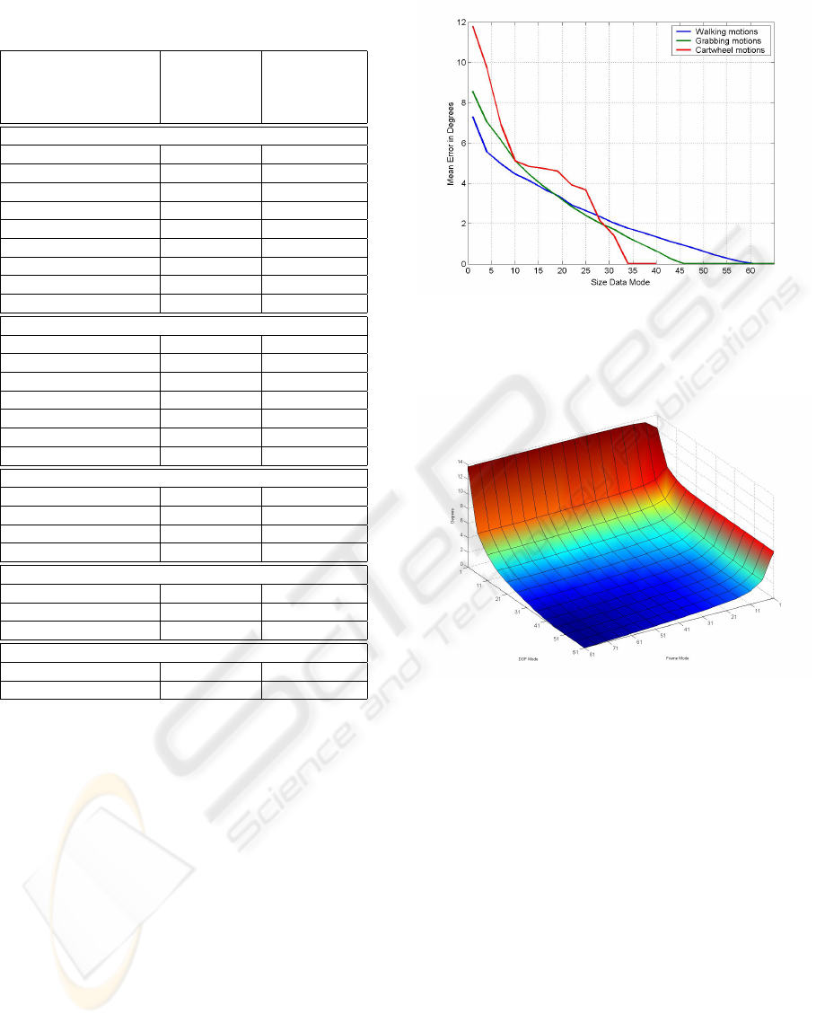
Table 1: Dimension, mean errors and size of the core tensor

for walking motions, represented by Euler angles.

Dimension Mean error Entries

Core Tensor walking Core Tensor

motions

(degrees)

Truncated Data Mode

5022 × 5 × 4 × 3 0.0 301320

64 × 5 × 4 × 3 0.0 3840

61 × 5 × 4 × 3 0.0 3660

58 × 5 × 4 × 3 0.1 3480

55 × 5 × 4 × 3 0.3 3300

40 × 5 × 4 × 3 1.3 2400

25 × 5 × 4 × 3 2.6 1500

10 × 5 × 4 × 3 4.4 600

1 × 5 × 4 × 3 7.3 60

Truncated DOF Mode

62 × 81 × 5 × 4 × 3 0.0 301320

52 × 81 × 5 × 4 × 3 0.0 252720

40 × 81 × 5 × 4 × 3 0.2 194400

31 × 81 × 5 × 4 × 3 0.8 150660

22 × 81 × 5 × 4 × 3 1.5 106920

10 × 81 × 5 × 4 × 3 3.8 48600

1 × 81 × 5 × 4 × 3 11.2 4860

Truncated Actor Mode

62 × 81 × 4 × 4 × 3 3.1 241056

62 × 81 × 3 × 4 × 3 5.2 180792

62 × 81 × 2 × 4 × 3 6.8 120528

62 × 81 × 1 × 4 × 3 9.4 60264

Truncated Style Mode

62 × 81 × 5 × 3 × 3 4.0 225990

62 × 81 × 5 × 2 × 3 5.6 150660

62 × 81 × 5 × 1 × 3 7.7 75330

Truncated Repetition Mode

62 × 81 × 5 × 4 × 2 2.1 200880

62 × 81 × 5 × 4 × 1 4.7 100440

4.1.1 Truncating Technical Modes

For our truncation experiments we systematically

truncated a growing number of components of the

core-tensors and reconstructed all motions. The mean

difference between all reconstructed and original mo-

tions – depending on the size of the truncated core-

tensor—is shown in table 1. The considered motions

were warped to a length of 81 frames and our skele-

ton, based on Euler angles, has 62 degrees of free-

dom. On this basis the resulting data tensor has a size

of 5022 × 5 × 4 × 3. The resulting core tensor after

applying an N-Mode SVD was now reduced. In ﬁg-

ure 3 the mean error E over all motions and all frames

is shown graphically in dependence of the size of the

Data Mode (blue). This error is deﬁned as follows:

E = (

Frames

DOFS

abs(e

org

i,j

− e

rec

i,j

))/(Frames · DOFS),

Figure 3: Mean error of reconstructed walking (blue), grab-

bing (green) and cartwheel (red) motions, depending on the

size of the Data Mode of the core tensor.

Figure 4: Displacement in degrees for truncated Frame and

DOF Mode.

where Frames is the number of all frames of all mo-

tions that were used to build the data tensor, and

DOFS is the number of degrees of freedom of the

underlying skeleton. This error is always calculated

on Euler angles hence the motions are stored in the

ASF/AMC ﬁle format.

One can see that the motions are reconstructed

without any visible error with no more than 61 of the

original 5022 dimensions.

If the technical Data Mode is split up into the

Frame and DOF Mode it is possible to make a sim-

ilar experiment by truncating both modes. The result

is shown in ﬁgure 4. If just the DOF Mode is trun-

cated the motion is reconstructed with a mean error

of less than one degree for more than 26 degrees of

freedom. The same displacement can be reached by

reducing the Frame Mode down to a size of 20.

MULTI-MODE REPRESENTATION OF MOTION DATA

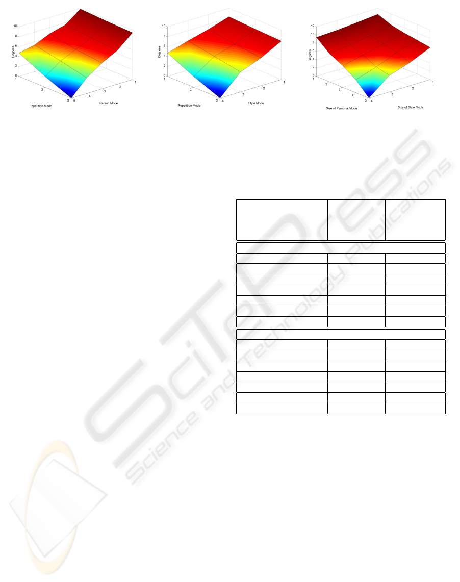
Figure 5: Mean error, in degrees, of reconstructed motions where two natural Modes were truncated. Style and Repetition

Mode are truncated (left). Personal and Repetition Mode are truncated (middle). Style and Personal Mode are truncated

(right).

4.1.2 Truncating Natural Modes

To verify the importance of natural modes we pro-

ceeded in the same way. In fact the displacement is

at the lowest size for the Repetition Mode. This is

what one would expect since the actors were asked to

perform the same action multiple times. The reason

for the observed displacement, is given through the

different interpretations of the motions. Note that sev-

eral interpretations from one actor are giving a smaller

variance, than motions from different actors or mo-

tions in different styles. The results of these experi-

ments are shown in ﬁgure 5. The displacement grows

higher with the size of truncated values from Style-

and Personal Mode.

4.2 Grabbing Motions

For this motion class the actors, which have been

the same as for the walking motions, were asked to

perform grabbing motions from a storage rack. The

Style Mode is derived from three different heights

(low, middle, and high). We took three takes of all

motions, that the repetition-mode has a size of three.

All grabbing motions were performed with the right

hand. Again all motions were warped to the length of

one reference motion. The data tensor has a size of

f · dof × 5 × 3 × 3. The resulting error for truncated

components of the Data Mode is shown in ﬁgure 3

(green).

4.3 Cartwheel Motions

The last class of motions we considered are cartwheel

motions. We captured several cartwheels from

four persons. All actors were asked to start their

cartwheels with the left foot and the left hand. We did

not deﬁne different “styles” for cartwheel motions.

The core tensor had a size of 6138 × 4 × 1 × 3. Here

Table 2: Dimension, mean errors and size of the core tensor

for grabbing motions, represented with Euler angles.

Dimension Mean error Entries

Core Tensor grabbing Core Tensor

motions

(degrees)

Truncated Data Mode

4340 × 5 × 3 × 3 0.0 195300

58 × 5 × 3 × 3 0.0 2610

55 × 5 × 3 × 3 0.0 2475

40 × 5 × 3 × 3 0.6 1800

25 × 5 × 3 × 3 2.4 1500

10 × 5 × 3 × 3 5.1 450

1 × 5 × 3 × 3 8.6 45

Truncated DOF Mode

62 × 70 × 5 × 3 × 3 0.0 195300

52 × 70 × 5 × 3 × 3 0.0 163800

40 × 70 × 5 × 3 × 3 0.3 126000

31 × 70 × 5 × 3 × 3 0.9 97650

22 × 70 × 5 × 3 × 3 1.9 69300

10 × 70 × 5 × 3 × 3 4.4 31500

1 × 70 × 5 × 3 × 3 9.7 3150

all motions could be reconstructed without any visi-

ble error for a size of no more than 34 for the Data

Mode. This results are shown in table 4.3 and can be

seen graphically in ﬁgure 3 (red).

4.4 Comparison with PCA

To compare our multi-linear model with linear mod-

els, as they are used for principal component analysis

(PCA), we constructed two tensors for our model and

two matrices for the PCA based on the same motions.

Figure 6 shows a comparison of the results for walk-

ing (left) and grabbing motions (right). The mean er-

ror over all reconstructed motions depending on the

number of principal components and the size of the

DOF Mode is shown in this ﬁgure. The mean error for

motions reconstructed from the multi-mode-model is

GRAPP 2007 - International Conference on Computer Graphics Theory and Applications

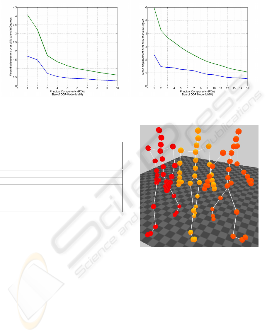
Figure 6: Mean error of reconstructed motions with reconstructions based on our model (blue) and based on a PCA (green).

The result is shown for walking motions (left) an d grabbing motions (right).

Table 3: Dimension, mean errors and size of the core tensor

for cartwheel motions, represented by Euler angles.

Dimension Mean error Entries

Core Tensor cartwheel Core Tensor

motions

(degrees)

Truncated Data Mode

6138 × 4 × 1 × 3 0.0 73656

34 × 4 × 1 × 3 0.0 408

31 × 4 × 1 × 3 1.4 372

16 × 4 × 1 × 3 4.4 192

1 × 4 × 1 × 3 11.8 12

smaller than the error from the motions reconstructed

from principal components. Thus a motion can be re-

constructed with a mean error less than one degree

above the complete motion from a core tensor when

the DOF Mode is truncated to just three components.

Thus especially in cases when a motion should be

approximated by rather few components the reduction

based on the multi-linear model is considerably better

than the one done by PCA.

4.5 Motion Synthesis

As it was described in Sect. 2.4, it is possible to syn-

thesize motions with our multi-linear model. For ev-

ery mode i there is an appropriate matrix U

, where

every row u

i,j

represents one of the motions j, this

mode consists of. Therefore an inter- or extrapolation

can be done between any rows of U before they are

multiplied with the core tensor Φ to synthesize a mo-

tion. To prevent our results from unrequested effects

like turns and unexpected ﬂips resulting from a repre-

Figure 7: Screenshot from the original motions that are

from the styles walking forward (red) and walking a left

circle (orange), the synthetic motion (yellow) is produced

by a linear combination of these styles.

sentation based on Euler angles we used our quater-

nion based representation to synthesize motions.

For the following walking example we con-

structed a motion that was interpolated between two

different styles. The ﬁrst style was walking four steps

straight forward and the second one was walking four

steps on a left round. We made a linear interpolation

by multiplying the corresponding rows with the factor

0.5. The result is a four step walking motion that de-

scribes a left round, with a larger radius. One sample

frame of this experiment can be seen in ﬁgure 7. An-

other synthetic motion was made by an interpolation

MULTI-MODE REPRESENTATION OF MOTION DATA

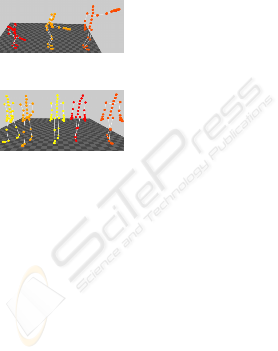
Figure 8: Screenshot from the original motions that are

from the styles grabbing low (red) and grabbing high (or-

ange), the synthetic motion (yellow) is produced by a linear

combination of these styles.

Figure 9: Screenshot from four original walking motions

and one synthetic motion, that is an result of combining two,

the personal and the style mode. The original motions of

the ﬁrst actor are on the left side, the original motions of the

second actor are on the right side and the synthetic example

can be seen in the middle.

of grabbing styles. We synthesized a motion by an

interpolation of the styles grabbing low and grabbing

high. The result is a motion that grabs in the mid-

dle. One result of this synthetic motion is shown in

ﬁgure 8.

With this technique we are able to make interpo-

lation between all modes parallel. One example is a

walking motion that is an interpolation between the

style and actors Mode. One picture of this result is

given in ﬁgure 9.

For more detailed results of our motion synthesis

we refer to the video.

5 CONCLUSION AND FUTURE

WORK

We have shown that exploring naturally occur-

ring modes in motion databases and representing

motions in multi-linear models—after appropriate

preprocessing—is a feasible way to represent mo-

tions of a database allowing different synthesis, anal-

ysis and compression of the motions. We expect that

multi-mode representations will be either an interest-

ing alternative or an additional toolkit in basically all

cases, in which currently principal component analy-

sis is used. As has been shown by our experiments,

the beneﬁt of the multi-linear representation over a

simply linear representation of a suitably structured

collection of motion data is especially relevant if mo-

tions should be approximated by rather few compo-

nents, e.g. in the context of reconstruction of motion

by low-dimensional control signals (Chai and Hod-

gins, 2005) or in the context of auditory presentation

of a motion (Droumeva and Wakkary, 2006; R

ober

and Masuch, 2005; Effenberg et al., 2005). This pa-

per presents a proof of concept, for which we could

use a motion database having examples for all data

of the built tensors. In general one might only have

sparsely given data for the different modes. However,

we presume that techniques similar to the ones used

to ﬁll the data tensors in the case of faces from sparse

data (Vlasic et al., 2005) can be used for motion data,

too. It will be a topic of our future research to inves-

tigate these techniques and to apply the multi-mode

representation to some of the tasks mentioned above.

ACKNOWLEDGEMENTS

We are grateful to Bernd Eberhardt and his group of

Hochschule der Medien in Stuttgart for the possibility

to build a systematic motion capture data base, which

is underlying our empirical investigations. Meinard

uller and Tido R

oder have not only been driving

forces behind the idea of building such a data base

but also contributed to its realization in many ways

– from serving as some of the actors to transforming

motion ﬁles into a well organized data base of motion

clips.

REFERENCES

Arikan, O. (2006). Compression of motion capture

databases. ACM Trans. Graph., 25(3):890–897. SIG-

GRAPH 2006.

Barbi

c, J., Safonova, A., Pan, J.-Y., Faloutsos, C., Hodgins,

J. K., and Pollard, N. S. (2004). Segmenting mo-

tion capture data into distinct behaviors. In Proceed-

ings of the 2004 conference on Graphics interface,

pages 185–194. Canadian Human-Computer Commu-

nications Society.

Bruderlin, A. and Williams, L. (1995). Motion signal pro-

cessing. In Proceedings of the 22nd annual con-

ference on Computer graphics and interactive tech-

niques, pages 97–104. ACM Press.

C. A. Andersson and R. Bro (2000). The N-way Toolbox

for MATLAB. http://www.models.kvl.dk/

source/nwaytoolbox/.

GRAPP 2007 - International Conference on Computer Graphics Theory and Applications

Carnegie Mellon University Graphics Lab (2004). CMU

Motion Capture Database. mocap.cs.cmu.edu.

Chai, J. and Hodgins, J. K. (2005). Performance animation

from low-dimensional contr ol signals. ACM Trans.

Graph., 24(3):686–696. SIGGRAPH 2005.

Droumeva, M. and Wakkary, R. (2006). Sound intensity

gradients in an ambient intelligence audio display. In

CHI ’06 extended abstracts on Human factors in com-

puting systems, pages 724–729, New York, NY, USA.

ACM Press.

Effenberg, A., Melzer, J., Weber, A., and Zinke, A. (2005).

MotionLab Sonify: A framework for the soniﬁcation

of human motion data. In Ninth International Confer-

ence on Information Visualisation (IV’05), pages 17–

23, London, UK. IEEE Press.

Giese, M. A. and Poggio, T. (2000). Morphable models for

the analysis and synthesis of complex motion patterns.

International Journal of Computer Vision, 38(1):59–

73.

Glardon, P., Boulic, R., and Thalmann, D. (2004). Pca-

based walking engine using motion capture data. In

CGI ’04: Proceedings of the Computer Graphics In-

ternational (CGI’04), pages 292–298, Washington,

DC, USA. IEEE Computer Society.

Hsu, E., Pulli, K., and Popovi

c, J. (2005). Style translation

for human motion. ACM Trans. Graph., 24(3):1082–

1089. SIGGRAPH 2005.

Kovar, L. and Gleicher, M. (2003). Flexible automatic mo-

tion blending with registration curves. In Breen, D.

and Lin, M., editors, Eurographics/SIGGRAPH Sym-

posium on Computer Animation, pages 214–224. Eu-

rographics Association.

Kovar, L. and Gleicher, M. (2004). Automated extraction

and parameterization of motions in large data sets.

ACM Transactions on Graphics, 23(3):559–568. SIG-

GRAPH 2004.

Kovar, L., Gleicher, M., and Pighin, F. (2002). Motion

graphs. ACM Transactions on Graphics, 21(3):473–

482. SIGGRAPH 2002.

Lee, J. and Shin, S. Y. (2002). General construction of time-

domain ﬁlters for orientation data. IEEE Transactions

on Visualizatiuon and Computer Graphics, 8(2):119–

128.

Majkowska, A., Zordan, V. B., and Faloutsos, P. (2006).

Automatic splicing for hand and body animations.

In ACM SIGGRAPH / Eurographics Symposium on

Computer Animation, pages 309–316.

Mukai, T. and Kuriyama, S. (2006). Multilinear motion

synthesis using geostatistics. In ACM SIGGRAPH /

Eurographics Symposium on Computer Animation -

Posters and Demos, pages 21–22.

Ormoneit, D., Black, M. J., Hastie, T., and Kjellstr

om,

H. (2005). Representing cyclic human motion us-

ing functional analysis. Image Vision Comput.,

23(14):1264–1276.

Robbins, K. L. and Wu, Q. (2003). Development of a com-

puter tool for anthropometric analyses. In Valafar,

F. and Valafar, H., editors, Proceedings of the Inter-

national Conference on Mathematics and Engineer-

ing Techniques in Medicine and Biological Sciences

(METMBS’03), pages 347–353, Las Vegas, USA.

CSREA Press.

ober, N. and Masuch, M. (2005). Playing Audio-only

Games: A compendium of interacting with virtual, au-

ditory Worlds. In Proceedings of Digital Games Re-

search Conference, Vancouver, Canada.

Safonova, A. and Hodgins, J. K. (2005). Analyzing the

physical correctness of interpolated human motion.

In SCA ’05: Proceedings of the 2005 ACM SIG-

GRAPH/Eurographics symposium on Computer ani-

mation, pages 171–180, New York, NY, USA. ACM

Press.

Safonova, A., Hodgins, J. K., and Pollard, N. S. (2004).

Synthesizing physically realistic human motion in

low-dimensional, behavior-speciﬁc spaces. ACM

Transactions on Graphics, 23(3):514–521. SIG-

GRAPH 2004.

Troje, N. F. (2002). Decomposing biological motion: A

framework for analysis and synthesis of human gait

patterns. Journal of Vision, 2(5):371–387.

Vlasic, D., Brand, M., Pﬁster, H., and Popovi

c, J. (2005).

Face transfer with multilinear models. ACM Trans.

Graph., 24(3):426–433. SIGGRAPH 2005.

Zinke, A. and Mayer, D. (2006). Iterative multi scale dy-

namic time warping. Technical Report CG-2006-1,

Universit

at Bonn.

MULTI-MODE REPRESENTATION OF MOTION DATA