
VOLUMETRIC SNAPPING:
WATERTIGHT TRIANGULATION OF POINT CLOUDS
Tim Volodine
1
, Michael S. Floater
2
and Dirk Roose
1
1
KULeuven, Department of Computer Science, Celestijnenlaan 200A, 3001 Heverlee, Belgium
2
CMA/IFI, University of Oslo, P.O.Box 1053 Blindern, 0316 Oslo, Norway
Keywords:
Meshing, surface reconstruction, volumetric grid, contouring, point clouds.
Abstract:
We propose an algorithm which constructs an interpolating triangular mesh from a closed point cloud of
arbitrary genus. The algorithm first constructs an intermediate structure called a Delaunay cover, which forms
a barrier between the inside and the outside of the object. This structure is used to build a boolean voxel
grid, with cells intersecting the cover colored black and all other cells colored white. The outer surface of the
voxel grid is snapped to the point cloud by replacing each exterior surface vertex with the closest point in the
point cloud. The snapped mesh is processed such that it is manifold and consists of triangles with good aspect
ratio. We show that if a fine voxel grid is used, the snapping yields Delaunay-like triangulation of the original
points. High grid resolutions are possible because of the Delaunay cover and a new contouring method, which
extracts the outer surface of the grid with O(n
2
) worst case space complexity, where n is the number of voxels
in one dimension.
1 INTRODUCTION
Nowadays 3D laser scanners are widely used to dig-
itize real-world objects for visualisation, reverse en-
gineering, inspection and animation. They produce
huge amounts of point data, sampled from the surface
of an object. While there are upcoming techniques for
manipulating point data directly (Szeliski and Ton-
nesen, 1992; Pauly et al., 2006), the mesh represen-
tation still remains a widespread standard for manip-
ulating and exchanging geometrical data. Therefore,
the problem of approximating a point cloud with a
polygonal mesh is an active topic of research.
Most scanners produce a very dense set of sam-
ples, not all of which are required in the final mesh.
Therefore, to save time and space, an implicit vol-
umetric representation of the point cloud is often
used. Reconstruction algorithms based on the implicit
approach typically involve an approximation of the
signed distance function, which is supplied to an iso-
surfacing method, such as Marching Cubes algorithm
(Lorensen and Cline, 1987), to extract the mesh.
However, the construction of a signed distance
function requires an oriented point cloud, i.e. a point
cloud with consistently oriented normals. This kind
of information is usually not available, significantly
complicating the reconstruction process. Further-
more, in the presence of noise and overlapping scans,
the signed distance function often results in topologi-
cal artifacts as pointed out in (Hornung and Kobbelt,
2006; Wood et al., 2004). To overcome this problem,
a volumetric method that does not rely on a signed
distance function was proposed recently by Hornung
and Kobbelt (Hornung and Kobbelt, 2006). They for-
mulate the reconstruction problem as a minimal cut
problem of a spatial graph defined on a voxel grid rep-
resentation of the point cloud. The edges in the graph
are weighted by confidence values, which can be in-
terpreted as an unsigned pseudo-distance of a voxel to
the closest point sample.
In this paper we propose a new volumetric method
that is relatively simple to implement and gives good
results in practice. Like the method of (Hornung and
Kobbelt, 2006) we avoid computing a signed distance
function. The main idea is to snap the triangulated ex-
terior surface of the voxel grid to the point cloud. But
in order to obtain a watertight voxelization at vari-
ous resolutions we voxelize an intermediate structure,
which is a union of triangle fans defining a barrier be-
tween the inside and the outside of the point cloud.
Because the construction of this structure is based
53
Volodine T., S. Floater M. and Roose D. (2007).
VOLUMETRIC SNAPPING: WATERTIGHT TRIANGULATION OF POINT CLOUDS.
In Proceedings of the Second International Conference on Computer Graphics Theory and Applications - GM/R, pages 53-60
DOI: 10.5220/0002079800530060
Copyright
c
SciTePress
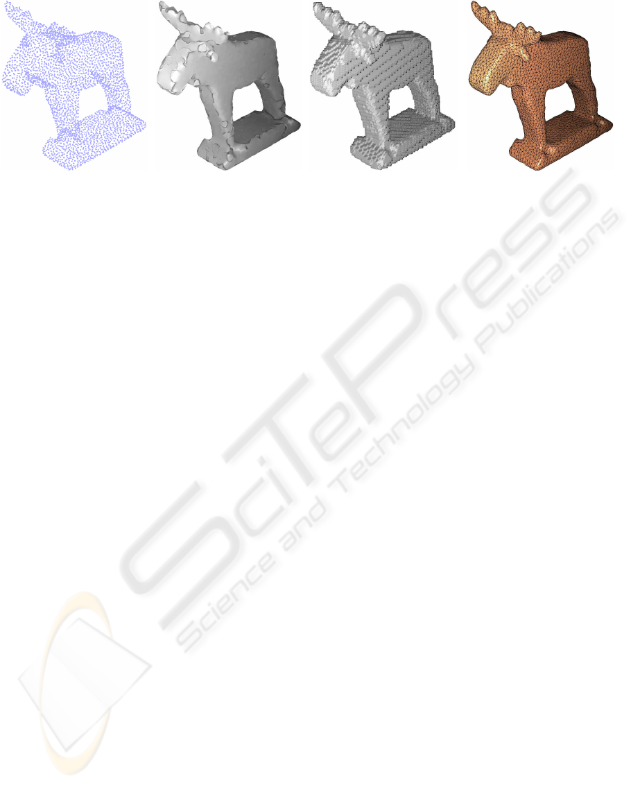
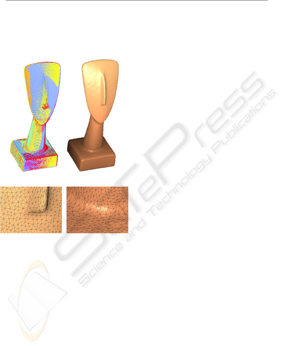
(a) (b) (c) (d)
Figure 1: The 4 main steps of the algorithm: (a) the Moose point cloud with 3K points (b) Delaunay cover (c) voxel grid (d)
mesh after snapping.
on Delaunay neighborhoods (Floater and Reimers,
2001), we call it a Delaunay cover of the point cloud.
The proposed algorithm guarantees a watertight
reconstruction, it can deal with noisy data or over-
lapping scans, and can reconstruct meshes of a large
number of points at various levels of detail. In addi-
tion our algorithm reconstructs convex sharp features
without any additional information, like the Hermite
data used in the Dual Contouring method (Ju et al.,
2002). Contrary to the traditional contouring algo-
rithms e.g. Marching Cubes and Dual Contouring,
the reconstructed mesh is interpolatory, with all the
vertices belonging to the original point cloud.
There are six conceptual steps in the proposed al-
gorithm: construction of the Delaunay cover, vox-
elization, triangulation, snapping, clean-up and opti-
mization. First, the Delaunay cover is constructed and
voxelized into a regular voxel grid. Each voxel is col-
ored either black (non-empty) or white (empty), de-
pending on whether it intersects the Delaunay cover
or not. Subsequently the exterior surface of the black
voxels is triangulated, yielding a first watertight ap-
proximation of the point cloud. This approximating
mesh is then snapped to the point cloud, with each
voxel corner replaced by the nearest point in the point
cloud. The snapping produces a geometric realisa-
tion of the voxel surface triangulation with the same
watertight topology. Since the snapping is in general
not injective, it yields degenerate and double trian-
gles. However, all such triangles are removed in a
simple clean-up step and this results in a valid man-
ifold mesh. Finally, when a coarse grid is used for
snapping, the obtained triangulation can be improved
by an optimization step. In this step the vertices are
diffused over the surface of the object in a manner
similar to the shrink-wrapping process of (Kobbelt
et al., 1999).
The task of triangulating the exterior voxel surface
is accomplished by a 2D tracing algorithm, which
processes the voxel grid slice by slice. The Delaunay
cover and the space efficient contouring algorithm al-
low to use small voxels. We show that, with increas-
ing grid resolution, the snapped triangulation con-
verges to Delaunay-like triangulation of the points.
2 RELATED WORK
Depending on the topology of the geometry (sam-
pling) of the point cloud, various methods for surface
reconstruction have been proposed in the literature.
We distinguish 4 main approaches: the implicit ap-
proach (Hoppe et al., 1992; Curless and Levoy, 1996;
Carr et al., 2001; Ohtake et al., 2003), methods based
on 3D Voronoi diagram (Amenta et al., 2001; Dey,
2006; Edelsbrunner and M
¨
ucke, 1994), advancing
front algorithms (Bernardini et al., 1999; Scheidegger
et al., 2005) and meshless parameterization (Floater
and Reimers, 2001; Zwicker and Gotsman, 2004).
Related to the snapping idea is the approach of
Kobbelt et al. (Kobbelt et al., 1999) for remeshing
genus-0 polygonal surfaces into meshes with subdi-
vision connectivity. The method simulates wrapping
of a plastic membrane around an object by starting
with a base mesh and iteratively applying projection,
smoothing and subdivision operators to it. In (Jeong
and Kim, 2002) Jeong et al. use the shrink-wrapping
approach to create a mesh of a genus-0 point cloud by
subdividing and shrink-wrapping its bounding box.
3 OVERVIEW
The algorithm consists of 6 steps,
GRAPP 2007 - International Conference on Computer Graphics Theory and Applications
54
1. Construct Delaunay Cover
2. Voxelize the Delaunay Cover
3. Triangulate the voxel grid surface
4. Snap the triangulated voxel surface to the point
cloud
5. Clean-up the triangulation (to obtain a manifold
triangulation)
6. (Optionally) optimize.
Note that the optimization step is only required when
the voxel grid is relatively coarse. In the following
sections we explain each of these steps in more detail.
4 DELAUNAY COVER
In order for the voxel surface to separate the inside
and the outside of the shape it needs to be closed. If
the voxelization is applied directly to the point cloud
it may result in holes in places where the sampling
density is larger than the grid size. To overcome this
problem we use an intermediate structure, called the
Delaunay cover of the point cloud. It consists of a
collection of triangles, which define a barrier between
the inside and the outside regions.
To explain the concept of a Delaunay Cover we
need a couple of definitions. First we need the no-
tion of the local planar Delaunay triangulation at p
i
,
which is the Delaunay triangulation of the projection
of the k nearest neighbors of p
i
on the tangent plane at
p
i
. The tangent plane is usually approximated by the
least squares plane through the k nearest neighbors.
The local planar Delaunay triangulation induces a lo-
cal triangulation at p
i
of the original k nearest neigh-
bors in the point cloud P.
Definition 1 (Delaunay Fan) A Delaunay fan
DFan(p
i
) of p
i
is the set of triangles in the local
triangulation of p
i
sharing p
i
as their common vertex.
Definition 2 (Delaunay Cover) Delaunay cover
DC(P) of a point cloud P is the union of all the
triangles in the Delaunay fans of each point in the
point cloud, i.e. DC(P) = ∪
p
i
∈P
DFan(p
i
).
In the planar case, when all points are in the plane
and no four of them are cocircular, the Delaunay cover
is simply the Delaunay triangulation of the points. In
3D the Delaunay cover approximates the point cloud,
but is neither a consistent triangulation, nor does it
have correctly oriented triangle normals, see figure
1(b).
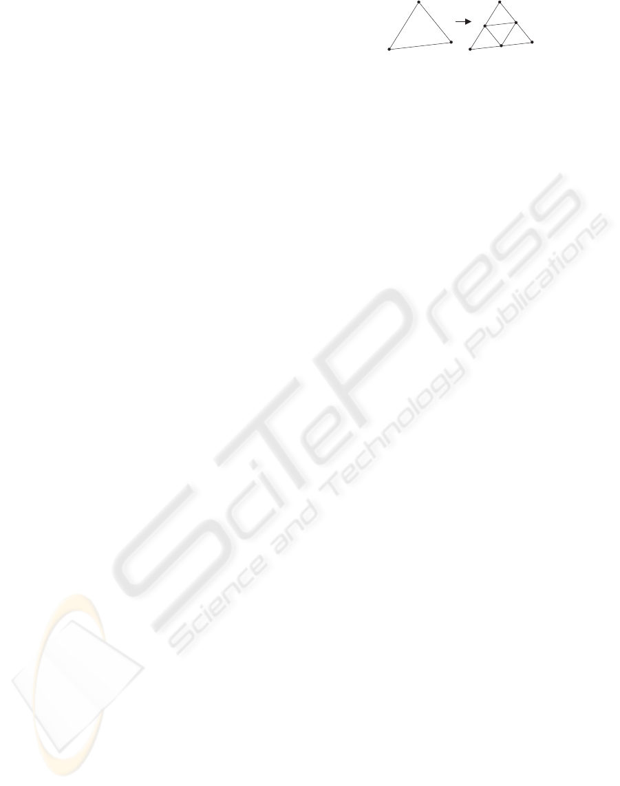
(a)
Figure 2: Refinement of the Delaunay cover : the triangle
is subdivided if one of its sides is longer than the voxel side
length. The new inserted vertices are the midpoints of the
triangle edges.
5 VOXELIZATION OF THE
DELAUNAY COVER
To voxelize the Delaunay cover into a regular voxel
grid, we could use the triangle-voxel intersection test.
In this approach a voxel is colored black if it is in-
tersected by a triangle and it is white otherwise. It
is possible to implement this kind of scan-conversion
efficiently using an octree and the Separating Axes
method for the intersection test, see (Ju, 2004). How-
ever in our algorithm we use a simpler technique to
color the voxels without computing intersections and
avoiding the construction of an octree.
5.1 Refinement of the Delaunay Cover
Let h be the voxel grid size (if the voxels are rect-
angular, let h be the minimal voxel edge length). In
order to obtain a proper voxelization, it is sufficient
to sample the Delaunay cover so that the distance be-
tween the sample points is smaller than h. The sam-
pled points can then be used to create a voxelization
in a straightforward way as explained later in 5.2.
To achieve the required sampling density we re-
fine the triangles in the Delaunay cover using a 1-
to-4 triangle split, as shown in figure 2. For each
triangle four new triangles are created if one of the
triangle sides is longer than h. The refinement is
performed iteratively until all triangles have sides of
length smaller than h. The refinement sequence can
be written as DC
0
(P) → DC
1
(P) → DC
2
(P) → . . . →
DC
κ
(P). With each DC
i
(P) there is an associated
point cloud P
i
.
5.2 Voxelization of the Refinement
The refinement of the Delaunay cover produces a set
of refined points P
κ
. To compute the voxel grid of this
point cloud, its bounding box, represented by the cor-
ners (x
min
, y
min
, z
min
)
⊤
and (x
max
, y
max
, z
max
)
⊤
, is di-
vided into cells of side length h. An example of such
a voxelization is shown in figure 1(c). In our imple-
mentation we use a boolean voxel grid, represented
VOLUMETRIC SNAPPING: WATERTIGHT TRIANGULATION OF POINT CLOUDS
55

+ +
Z
Y
X
=
Figure 3: The three stripes parallel to the XY-plane, XZ-
plane and YZ-plane are combined to obtain a triangulation
of the voxel.
by a 3D matrix V ∈ Z
n
x
×n
y
×n
z
2
, where n
x
, n
y
and n
z
is
the number of voxels in the corresponding dimension.
The matrix has a nonzero entry iff the corresponding
voxel contains at least one point p
i
= (x
i
, y
i
, z
i
) in P
κ
.
Starting with the zero matrix V, the voxelization is
obtained by setting
V
x
i
− x
min
h
,
y
i
− y
min
h
,
z
i
− z
min
h
= 1.
However, the memory consumption of this ap-
proach poses a problem, because the classical repre-
sentation of a 3D matrix grows as a cube of the num-
ber of cells in each dimension. Fortunately, the matrix
V will typically be very sparse, so the memory prob-
lem can be avoided by using a sparse representation
of V. Our sparse representation stores only the non-
zero entries in a hash table. This approach is both
extremely fast and memory efficient.
6 TRIANGULATION OF THE
VOXEL GRID SURFACE
We construct a consistent triangulation of the voxel-
grid by processing it slice by slice in 3 directions (X,
Y and Z). A slice is a 2D submatrix of V where one
of the 3 dimensions is fixed, e.g. the first horizon-
tal slice in the Z-direction is given by B = V(·, ·, 1).
As shown in figure 3 the cube (one voxel) is com-
pletely and consistently covered by overlaying three
triangle strips. The overlaid strips may cover some
of the voxel faces two times. This is easily resolved
by removing double triangles. For convex objects any
two striping directions are actually sufficient to cover
the whole surface. However for more complicated ob-
jects, e.g. the torus, we need 3 directions to be certain
that the whole grid surface is covered.
6.1 The Contouring Algorithm
The contouring algorithm operates on a slice of V,
which is a 2D submatrix B ∈ Z
n
x
×n
y
2
(if the slice is in
the Z-direction). It traces the contour counterclock-
wise around the nonzero (gray) entries in B, as shown
in figure 5(a). Starting with the rightmost non-empty
X
(a)
X
(b)
X
(c)
X
(d)
Figure 4: The four cases for the tracing algorithm.
cell, we start moving upwards and always keep the
gray cells to the left of the tracing direction.
The tracing algorithm can be implemented by ob-
serving that there are only 4 cases to consider during
tracing. They are depicted in figure 4. Imagine we are
at position X in the figure, having just traced the verti-
cal line below it. To decide where to go next we need
to look at the content of the four neighboring cells.
The four cases in the figure are the possible cases, all
other configurations can be reduced to these 4 cases
by rotation.
The traced 2D contour is used to create a triangu-
lation of the outer surface of the slice. We create 2
parallel contours in 3D by lifting the traced 2D con-
tour to 3D and offsetting it with the cell size in the
third dimension. The outer surface of the slice is the
quad strip of voxel faces contained between two con-
tours. These voxel faces are triangulated by connect-
ing the corresponding points (see figure 3).
If B contains multiple contours, they are extracted
by applying the tracing algorithm multiple times.
Each time a contour is extracted all the cells it en-
closes are filled with zeros and the tracing algorithm
is repeated.
6.2 Contouring Cropped Grids
The contouring algorithm can be extended to handle
holes lying on the boundaries of the bounding box.
This extension allows the reconstructed mesh to be
cropped by shrinking the bounding box. In order for
the contouring algorithm to work with holes, the orig-
inal matrix B is augmented with a boundary layer of
non-empty entries. When applying the tracing algo-
rithm in the presence of a hole, it produces a dual con-
tour as shown in figure 5(b). The final contour is ob-
tained by removing the traced segments between c
1
and c
2
.
7 SNAPPING
Voronoi diagrams can be constructed by adaptively
subdividing and sampling the space using an octree
(or a quadtree in 2D), see e.g. (Lavender et al., 1992;
Boada et al., 2002). This approach is especially useful
for approximating the generalized Voronoi diagram,
GRAPP 2007 - International Conference on Computer Graphics Theory and Applications
56
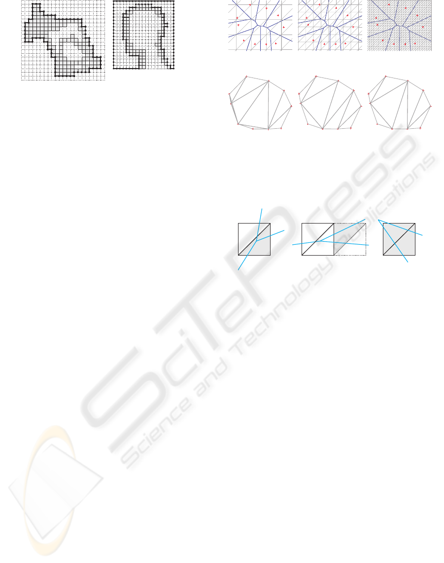
(a)
c
1
c
2
(b)
Figure 5: (a) contour of a slice of the moose (b) dual contour
of the slice of the mannequin head model with a hole.
where the sites are geometric primitives other than
points.
Snapping the corners of a uniform triangulated
grid to the closest points in the data set has a sim-
ilar effect to the space sampling approach. In the
following paragraph we show that snapping can be
used to construct a Delaunay triangulation (the dual
of the Voronoi diagram) of points in the plane. In 3D
we sample the space in the vicinity of the Delaunay
cover using voxel corners. If the voxels are smaller
than the inter-point distances in the point cloud, we
obtain an effect similar to the 2D situation, leading to
a Delaunay-like triangulation of the surface points.
7.1 Delaunay Triangulation
Figure 6 illustrates the snapping algorithm in the
plane. The red sample points are overlaid with trian-
gulated grids (figures 6(a)-6(c)) with increasing res-
olutions. Figures 6(d)-6(f) show the resulting trian-
gulations after snapping each grid point to the closest
red point. Coarse grids produce a triangulation with
overlapping triangles, or miss some of the original red
points (figures 6(d) and 6(e)). Fine grids result in the
Delaunay triangulation of the red points (figure 6(f)).
The triangulation is actually the Delaunay triangula-
tion plus various degenerate and repeated triangles,
but these extra triangles are easy to remove.
To state a sufficient condition for obtaining the
Delaunay triangulation we analyse the Voronoi di-
agram of the red points (e.g. figure 6(a)). In the
Voronoi diagram we call two Voronoi cells neighbors
if they share an edge. We define the distance between
two cells as the shortest distance between any two
points lying on the boundary of these cells. In this
way the distance between neighboring cells is zero.
The sufficient condition for obtaining the Delau-
nay triangulation by snapping the grid is that the grid
diagonals (longest triangle side) should be smaller
than the distance between any two non-neighboring
Voronoi cells. This condition also implies that degen-
erate cases, such as 4 or more points lying on a circle,
(a) (b) (c)
(d) (e) (f)
Figure 6: (a) cell size=0.6 (b) cell size=0.31 (c) cell size=0.1
(d) triangulation corresponding to (a), note the overlapping
triangles; (e) triangulation corresponding to (b); (f) triangu-
lation corresponding to (c), this is the Delaunay triangula-
tion.
(a) (b) (c)
Figure 7: The three possible configurations in the snap-
ping algorithm which yield non-degenerate triangles: (a)
the gray triangle is snapped to a Delaunay triangle corre-
sponding to the Voronoi vertex inside the grid cell (b) the
gray triangle is snapped to the Delaunay triangle corre-
sponding to the Voronoi vertex in the neighboring cell (c)
both gray triangles are snapped to the same Delaunay tri-
angle corresponding to the Voronoi vertex outside the grid
cell.
cannot be Delaunay triangulated with the snapping
algorithm, because in that case the distance between
non-neighboring cells is zero.
To see why this condition is true we analyse the
possible configurations of the grid cells w.r.t. the
Voronoi diagram. Under above condition there are
only three essential configurations which yield non-
degenerate triangles after snapping. These cases are
shown in figure 7. All three cases create only Delau-
nay triangles, sometimes multiple times (as in figure
7(c)).
8 CLEAN-UP
After snapping, the resulting triangulation is usually
not a topologically manifold triangulation. By topo-
logically manifold we mean that each point has a fan
of triangles homeomorphic to a disc and each edge is
VOLUMETRIC SNAPPING: WATERTIGHT TRIANGULATION OF POINT CLOUDS
57
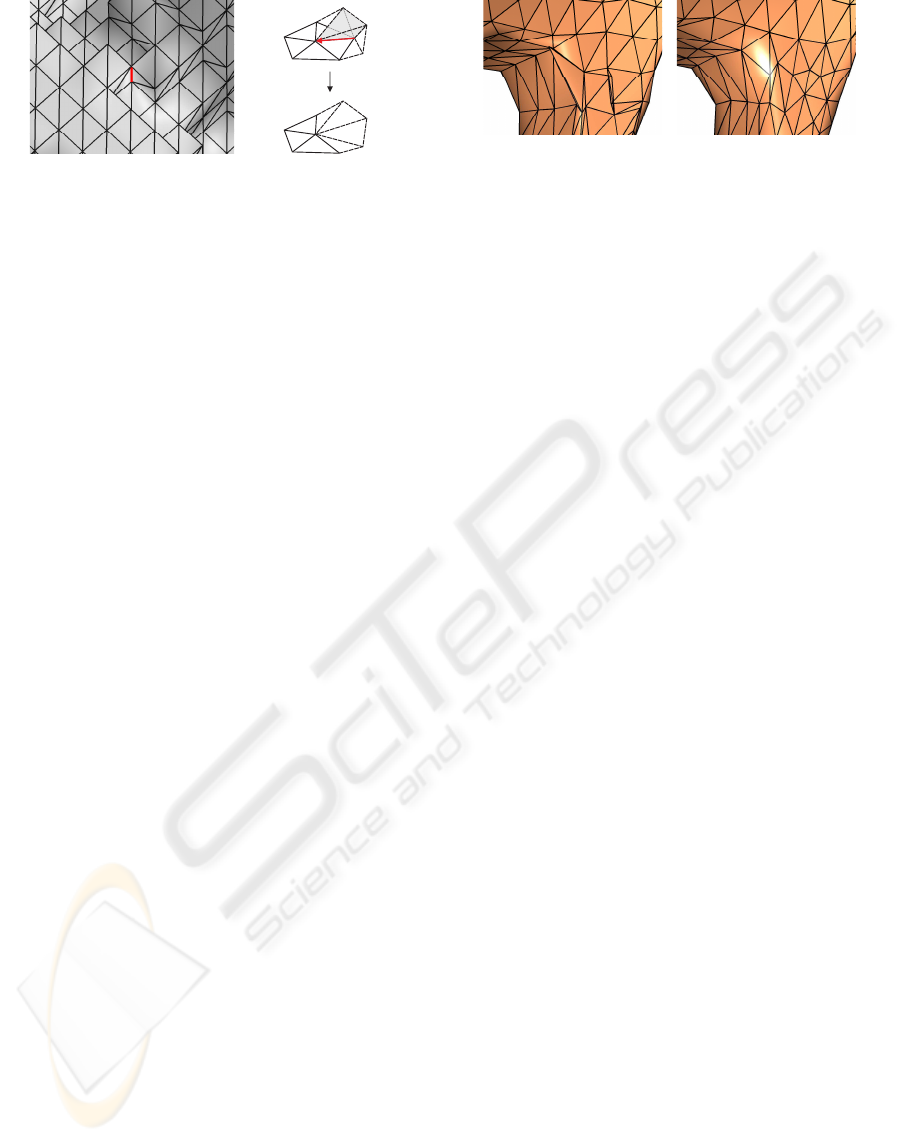
(a) (b)
Figure 8: (a) non-manifold edge on the outer surface of the
voxel grid (b) collapse of a non-manifold edge.
shared exactly by two triangles. During the clean-up
step we process the triangles such that the result is a
manifold triangulation.
To obtain a manifold triangulation we remove the
following items (in this order):
1. degenerate triangles (having at least two coincid-
ing vertices)
2. multiple triangles (having the same vertices)
3. dangling triangles (which do not have three neigh-
boring triangles)
4. non-manifold edges (edges shared by more than
two triangles)
A degenerate triangle is created when two or three
vertices of a voxel triangle are snapped to the same
data point. Double triangles arise in cases as shown
in figure 7(c). The removal of the first two items can
occasionally result in dangling triangles, which are
simply deleted from the triangulation. In some rare
cases the triangulation of the exterior surface of the
voxel grid can contain non-manifold edges, as shown
on figure 8(a). To remove the non-manifold edges we
collapse them, by snapping one end of the edge to
the other, as shown in figure 8(b). Note that an edge
collapse introduces degenerate and double triangles,
which are cleaned up by executing the first three items
once more.
9 OPTIMIZATION
The optimization step is only required when the voxel
grid is coarse relative to the inter-point distance in the
point cloud. The idea of the optimization step is to
diffuse the vertices over the surface such that the po-
sition of each vertex is approximately at the center of
its neighbors. The optimization is performed for two
reasons. On the one hand, it improves the mesh qual-
ity and yields triangles with better aspect ratio. On the
other hand, it unfolds locally folded triangles, which
can occasionally appear after the snapping of coarse
grids. Such triangles typically have a normal which is
(a) (b)
Figure 9: Illustration of how the smooth-snap iteration re-
solves folded triangles; (a) folded triangles near the leg of
the moose (b) mesh after one smooth-snap iteration.
in the opposite direction to the normals of the neigh-
boring triangles (figure 9(a)).
The optimization process is a number of smooth-
snap iterations, consisting of two steps:
1. Smooth the manifold mesh and
2. Re-snap the smoothed mesh onto the point cloud.
In practice 1 or 2 iterations already give a significant
improvement of the triangulation. We implemented
the smoothing step using the simplest possible ap-
proach, i.e. Laplacian smoothing, where each ver-
tex in the triangulation is replaced by the centroid of
its neighbors. To obtain better diffusion we swap the
edges in the 1-ring neighborhoods of vertices with va-
lency 4, but only when no new valency 4 vertices are
created by the edge swap.
10 RESULTS AND DISCUSSION
We applied the proposed meshing algorithm to differ-
ent kinds of points clouds. The Moose point cloud
(figure 1) is uniformly sampled. The Mannequin
Head (figure 12) has adaptive sampling density, with
more points in places of high curvature. In addition it
illustrates the ability of the algorithm to handle point
clouds with boundaries. Finally, the Cycladic Head
model (figure 11) consists of a number of overlapping
registered scans.
For both the Moose and the Mannequin Head data
sets we used fine voxel grids without the optimization
step (figures 12 and 1). Table 10 summarizes the algo-
rithm statistics for the Moose model containing 10K
points for different grid sizes. Note that there are no
folded triangles for the finest grid resolution. We used
a relatively coarse grid for the Cycladic Head model,
followed by two smooth-snap optimization steps (fig-
ure 11).
The algorithm was implemented in C++ and exe-
cuted on an Pentium 4 2.4Ghz machine with 512MB
of RAM. The total time for the Moose 3K model
was 4.8s, with the contouring step consuming 70% of
the time. The Cycladic Head required a total of 76s,
GRAPP 2007 - International Conference on Computer Graphics Theory and Applications
58
grid size DC-refinement # grid vertices nm edges
1
degenerate double dangling # folds
2
final
3
14× 21× 22 – 1010 0 52 0 0 34 984
49× 78× 82 43597 13759 7 9048 127 121 395 9116
120× 192× 202 208674 82948 1 144718 147 78 0 10502
1
– number of non-manifold edges
2
– number of folded fans
3
– number of points in the final triangulation (after clean-up)
Figure 10: Statistics for the Moose 10K point cloud. Table shows the number of points, degenerate triangles, double triangles,
dangling triangles, folded triangles and the number of points in the final triangulation for different grid sizes.
(a) (b)
(c) (d)
Figure 11: (a) 9 aligned (registered) scans of the Cycladic
Head point cloud, each scan has a different color (in total
190K points) (b) resulting mesh on a 61× 97 × 102 grid,
14K points and 28K triangles (c) close-up of the nose of the
reconstructed mesh (d) close-up of the region near the socle
of the model.
with 31% of the time spent on the construction of the
Delaunay cover. The computation of the Delaunay
cover requires a parameter k for the number of near-
est neighbors. In our experience k ∈ [15, 25] yields
sufficient coverage for most point clouds. The snap-
ping step is implemented using an octree structure, so
that closest points can be located efficiently.
11 CONCLUSION
We found the method to work very well with real data
obtained from a 3D laser scanner as well as filtered
point clouds. It allows the construction of interpo-
lating triangulations with various levels of detail by
choosing the voxel size h. In order to obtain a closed
voxelization we introduce the concept of a Delaunay
cover. For filtered point clouds the Delaunay cover
allows the use of small h, resulting in high quality
triangulation of the points. For coarse grids the De-
launay cover may not be required, but in practice we
always compute the Delaunay cover, otherwise it is
difficult to determine the appropriate grid cell size. A
limitation of the method is that it cannot be applied to
point clouds with holes, unless the holes are aligned
with the boundaries of the bounding box.
In our implementation we perform the extraction
of the outer voxel surface by a 2D tracing algorithm,
requiring n
x
+ n
y
+ n
z
slices of the voxel grid. An
alternative is to use a 3D flooding algorithm, which
would require O((n
x
+ n
y
+ n
z
)
3
) storage, while our
contouring algorithm has quadratic storage complex-
ity.
ACKNOWLEDGEMENTS
We thank Martin Reimers for helpful discussions
and for providing his software for inspection of non-
manifoldness in triangulations. We thank the CMA,
Oslo, for the use of their 3D scanner to generate the
Moose and the Cycladic Head point clouds. This
work was partly supported by the Project IUAP P5/22
of the Belgian Science Policy Office and the BeMatA
program of the Norwegian Research Council.
REFERENCES
Amenta, N., Choi, S., and Kolluri, R. (2001). The power
crust, unions of balls, and the medial axis transform.
Computational Geometry: Theory and Applications,
19(2-3):127–153.
Bernardini, F., Mittleman, J., Rushmeier, H., Silva, C., and
Taubin, G. (1999). The ball-pivoting algorithm for
surface reconstruction. IEEE Transactions on Visual-
ization and Computer Graphics, 5(4):349–359.
VOLUMETRIC SNAPPING: WATERTIGHT TRIANGULATION OF POINT CLOUDS
59
Boada, I., Coll, N., and Sellar
´
es, J. (2002). Hierarchical pla-
nar voronoi diagram approximations. In Proceedings
of the 14th Canadian Conference on Computational
Geometry, pages 40–45.
Carr, J. C., Beatson, R. K., Cherrie, J., Mitchell, T. J.,
Fright, W. R., McCallum, B. C., and Evans, T. R.
(2001). Reconstruction and representation of 3d ob-
jects with radial basis functions. In ACM SIGGRAPH
2001, pages 67–76.
Curless, B. and Levoy, M. (1996). A volumetric method for
building complex models from range images. Com-
puter Graphics, 30(Annual Conference Series):303–
312.
Dey, T. K. (2006). Curve and Surface Reconstruction:
Algorithms with Mathematical Analysis. Cambridge
University Press.
Edelsbrunner, H. and M
¨
ucke, E. P. (1994). Three-
dimensional alpha shapes. ACM Transactions on
Graphics, 13(1):43–72.
Floater, M. and Reimers, M. (2001). Meshless parame-
terization and surface reconstruction. Comp. Aided
Geom. Design, 18:77–92.
Hoppe, H., DeRose, T., Duchamp, T., McDonald, J., and
Stuetzle, W. (1992). Surface reconstruction from un-
organized points. In ACM SIGGRAPH 1992, pages
71–78.
Hornung, A. and Kobbelt, L. (2006). Robust reconstruction
of watertight 3d models from non-uniformly sampled
point clouds without normal information. In Euro-
graphics Symposium on Geometry Processing, pages
41–50.
Jeong, W. and Kim, C. (2002). Direct reconstruction of dis-
placed subdivision surface from unorganized points.
In Graphical Models, volume 64(2), pages 78–93.
Ju, T. (2004). Robust repair of polygonal models. ACM
Trans. Graph., 23(3):888–895.
Ju, T., Losasso, F., Schaefer, S., and Warren, J. (2002).
Dual contouring of hermite data. ACM Trans. Graph.,
21(3):339–346.
Kobbelt, L. P., Vorsatz, J., Labsik, U., and Seidel, H.-P.
(1999). A shrink wrapping approach to remeshing
polygonal surfaces. In Computer Graphics Forum
(Eurographics ’99), volume 18(3), pages 119–130.
Lavender, D., Bowyer, A., Davenport, J., Wallis, A., and
Woodwark, J. (1992). Voronoi diagrams of set-
theoretic solid models. IEEE Computer Graphics and
Applications, 12(5):69–77.
Lorensen, W. and Cline, H. (1987). Marching cubes: A high
resolution 3d surface construction algorithm. ACM
Trans. Graph., 21(4):163–170.
Ohtake, Y., Belyaev, A., Alexa, M., Turk, G., and Seidel,
H.-P. (2003). Multi-level partition of unity implicits.
ACM Trans. Graph., 22(3):463–470.
Pauly, M., Kobbelt, L. P., and Gross, M. (2006). Point-
based multiscale surface representation. ACM Trans.
Graph., 25(2):177–193.
Scheidegger, C., Fleishman, S., and Silva, C. (2005). Tri-
angulating point-set surfaces with bounded error. In
Proceedings of the third Eurographics Symposium on
Geometry Processing, pages 63–72.
Szeliski, R. and Tonnesen, D. (1992). Surface modeling
with oriented particle systems. In SIGGRAPH 1992,
Computer Graphics Proceedings, pages 185–194.
Wood, Z., Hoppe, H., Desbrun, M., and Schr
¨
oder, P. (2004).
Removing excess topology from isosurfaces. ACM
Trans. Graph., 23(2):190–208.
Zwicker, M. and Gotsman, C. (2004). Meshing point clouds
using spherical parameterization. In Proceedings of
the Eurographics Symposium on Point-Based Graph-
ics.
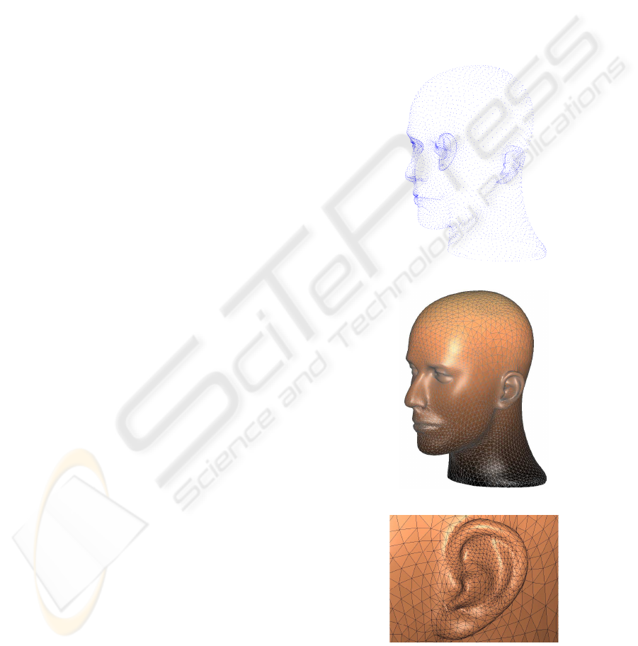
(a)
(b)
(c)
Figure 12: (a) point cloud of the Mannequin model (6K
points) (b) reconstructed mesh on a 190 × 253 × 301 grid
(c) closeup of the ear.
GRAPP 2007 - International Conference on Computer Graphics Theory and Applications
60
