MORPHOLOGY-BASED REPRESENTATIONS OF DISCRETE

SCALAR FIELDS

Mohammed Mostefa Mesmoudi

Department of Mathematics, Mostaganem University, Route Belhacel Po.Box 227, 27000 Mostaganem, Algeria

Leila De Floriani

Department of Computer Science, University of Genova, Via Dodecaneso n 35, 16146 Genova, Italy

Keywords:

Gradient vector ﬁeld, Morse theory, Geometric modeling, Smale decomposition, Forman theory.

Abstract:

Forman introduced in (Forman, 1998) a theory for cell complexes that is a discrete version of the well known

Morse theory. Forman theory ﬁnds several applications in digital geometry and image processing where

the data to be processed are discrete, see for instance (Lewiner et al., 2002a), (Lewiner et al., 2002b). In

(DeFloriani et al., 2002b), we have introduced a Smale-like decomposition of a scalar ﬁeld f deﬁned on a

triangulated domain M based on a discrete gradient ﬁeld that simulates well the behavior of the gradient ﬁeld

in the differentiable case. Here, we extend our discrete gradient vector ﬁeld so that the extended form coincides

with a Forman gradient ﬁeld. The extended gradient ﬁeld does not change the Smale-like decomposition

components and, thus, inherits properties of both smooth Morse and discrete Forman functions.

1 INTRODUCTION

Morse theory is a powerful tool for understanding the

topology and the geometry of a manifold on which

a C

-differentiable function is deﬁned. This theory

has been developed in the middle of the last cen-

tury by Thom, Morse, Milnor and Smale. Any C

differentiable function (with n ≥ 2) can be approxi-

mated with its derivatives by a Morse function, (Mil-

nor, 1963). Thom (Thom, 1949), followed by Smale

(Smale, 1960), has shown that a manifold M endowed

with a Morse function admits a CW representation

composed of cells, called stable( or unstable) man-

ifolds. Each cell is associated with a critical point

of the function. This decomposition is based on the

study of the behavior of the gradient vector ﬁeld of the

function. Another decomposition of the manifold into

handles can be performed by following the growth of

level sets of the function (Milnor, 1963). The topol-

ogy (i.e., the homotopy type) of the level sets changes

when a critical point is reached. Thus, critical points

have a crucial role in Morse theory.

For a discrete scalar ﬁeld, the ﬁeld values are known

only on a discrete set of points scattered over a grid

(regular or irregular). To study a scalar ﬁeld, an inter-

polation by a differentiable function is usually done,

(Watson et al., 1985) and (Nackman, 1984). Then,

Morse theory is used to extract critical points and

critical lines that bound the cells of a Morse com-

plex. This operation depends on the approximation

performed and is expensive in term of computation

time and memory space. To reduce that, other au-

thors tried to treat the data of a two-dimensional im-

age (Peucker and Douglas, 1975)and (J.Toriwaki and

Fukumura, 1975) by performing a local study around

each point. Other authors (Bajaj and Shikore, 1998),

(Bajaj et al., 1998) and (Edelsbrunner et al., 2001)

have interpolated the discrete data by piecewise lin-

ear functions, loosing, thus, the differentiability ad-

vantages.

In 1998, Forman introduced for cell complexes a

novel theory that is a discrete equivalent to Morse the-

ory (Forman, 1998). He has proven similar results to

those proven within the smooth Morse theory. For-

man theory handles the data discretely in a new way

differently from all the other methods known simu-

lating the differentiable case. Forman succeeded to

prove all the main theorems of smooth Morse the-

ory for discrete functions. Forman theory is ﬁnding

several applications in computer graphics (see, for in-

stance, (Lewiner et al., 2002b) and (Lewiner et al.,

2002a)).

137

Mostefa Mesmoudi M. and De Floriani L. (2007).

MORPHOLOGY-BASED REPRESENTATIONS OF DISCRETE SCALAR FIELDS.

In Proceedings of the Second International Conference on Computer Graphics Theory and Applications - GM/R, pages 137-144

DOI: 10.5220/0002080501370144

 SciTePress

In (DeFloriani et al., 2002b), we have intro-

duced a Smale-likedecomposition a of triangulated n-

dimensional domain M associated with a scalar ﬁeld

f. We deduced a discrete gradient vector ﬁeld Grad f,

which we have been used in (DeFloriani et al., 2002a)

to extract, and classify critical points and to extract

a discrete Morse decomposition that represents the

topology structure of the ﬁeld. We have shown in

(Danovaro et al., 2003) that our discrete gradient vec-

tor ﬁeld simulates well the behavior of the differen-

tiable gradient ﬁeld case.

Here, we construct an extended form of our dis-

crete gradient vector ﬁeld that corresponds to the gra-

dient ﬁeld of a Forman function F whose restriction

over vertices of M coincides with the initial scalar

ﬁeld f . We give the explicit formulation of Forman

function F that satisﬁes the above property. As a con-

sequence, we have that:

• All Forman results (speciﬁcally, simpliﬁcation

and compression process) can be applied to our

discrete scalar ﬁeld.

• For a triangulated embedded domain, not all the

values over the cells of a Forman function are

necessary to study the morphology of the domain.

Only values at the vertices are required.

• Differentiability simulation of the induced gra-

dient vector ﬁeld allows us to understand the

behavior of the corresponding Morse function

well, and hence its decomposition into stable and

unstable components.

• The compatibility of our extended gradient ﬁeld

with both smooth Morse and discrete Forman gra-

dient ﬁelds provides a powerful tool to handle

continuous and discrete properties at the same

time.

The remainder of this paper is organized as fol-

lows. In the next Section we summarize some results

relative to smooth functions, and we recall some com-

binatorial notions. In Section2, we present the main

properties of smooth Morse theory. In Section 4, we

report some results from Forman theory that we need

for our construction. In Section 5, we review brieﬂy

our Smale-like decompositionand we discuss some of

its properties. In Section 6, we present the construc-

tion of the process that extends our discrete gradient

vector ﬁeld to a Forman one. This proves the compat-

ibility of our Smale-like decomposition with Forman

theory. In the last section, we describe our on-going

work.

2 BACKGROUND

In this Section we recall some fundamental notions

on functions and some combinatorial notions that we

need in the remainder of the paper.

Let f be a differentiable real-valued function de-

ﬁned on a manifold M of dimension n. The gradient

of f at a point P ∈ M is a vector Grad

f tangent to M

at P that is deﬁned by the ﬁrst derivatives of f at P.

We have Grad

f = (

∂f

∂x

, . . . ,

∂f

∂x

), where (x

, . . . ,x

)

are local coordinates around P. The set of all gradi-

ent vectors in M is called the gradient vector ﬁeld of

f and denoted by Grad f. We say that P is a crit-

ical point of f if the gradient vector vanishes at P.

It is well known that the gradient vector ﬁeld indi-

cates the steepest direction in which the function is in-

creasing. Curves integrating the gradient vector ﬁeld

(i.e., everywhere tangent to the gradient vector ﬁeld)

are called integral curves. Integral curves follow the

(gradient) direction in which f has the maximal in-

creasing growth. Hence, integral curves cannot be

closed, nor inﬁnite (in a compact manifold), and they

do not self-intersect. They are emanating from critical

points, or from boundary components of the domain

and converge to other critical points, or to boundary

components.

Let now recall some combinatorial notions, for de-

tails we refer to (Agoston, 1976). Let k be an integer,

a k-simplex or a k- dimensional simplex is the con-

vex hull of (k+ 1) afﬁnely independent points, called

vertices. A face σ of a k-simplex γ, σ ⊆ γ, is a j-

simplex (0 ≤ j ≤ k) generated by ( j+1) vertices of γ.

A simplicial complex K is a collection of simplexes,

called also cells, such that if γ is a simplex in K, then

each face σ ⊆ γ is in K, and, the intersection of two

simplexes is either empty or a common face of them.

We call a top simplex in K a simplex which is not the

proper face of any simplex in K.

The carrier | K | of a simplicial complex K is the

space of all points in simplexes of K. In this case, K

is called a triangulation of | K |.

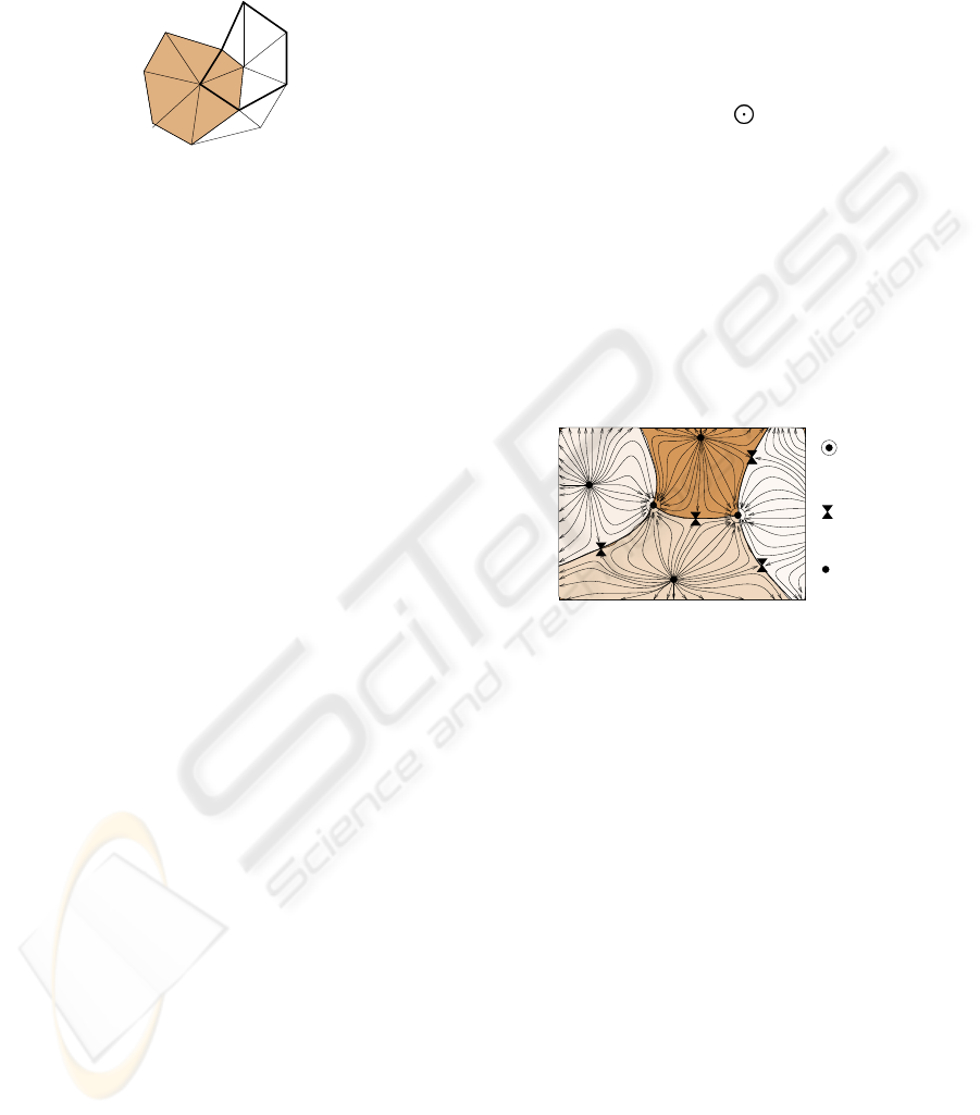
Let K be a simplicial complex and γ be a cell in K.

The star of γ is the set St(γ) of all cells in K which are

incident at γ. Thus, St(γ) = {σ ∈ K : γ ⊆ σ}. The star

of γ describes the neighborhood of γ in the complex

(see Figure 1(a)). The closure of a set of cells Γ is the

smallest subcomplex

Γ of K containing Γ. Clearly, Γ

consists of all cells of Γ plus their faces.

The link of cell γ is the subcomplex Lk(γ) of K

deﬁned as Lk(γ) = St(γ)−St(γ), where γ is the closure

of γ. The link describes the boundary of St(γ) (see

Figure 1(a)).

A cone from a vertex w to a simplex γ is the con-

vex combination of all vertices of γ with w. We denote

GRAPP 2007 - International Conference on Computer Graphics Theory and Applications

138

it by (γ, w). If w is afﬁnely independent of the vertices

of γ, then the cone from w to γ is a simplex of dimen-

sion dim(γ) + 1, where dim(γ) denotes the dimension

of γ.

(c)

Figure 1: The shaded region is the star of v. The graph in

bold is the link of the vertex w.

3 SMOOTH MORSE THEORY

A Morse function on a manifold M is a C

differentiable real-valued function f deﬁned on M

such that its critical points are non-degenerate (Mil-

nor, 1963). This means that the Hessian matrix

Hess

f of the second derivativesof f at any point P ∈

on which the gradient of f vanishes (Grad

f = 0)

is non-degenerate (Det(Hess

f 6= 0). Morse (Milnor,

1963) has proven that there exists a local coordinate

system (y

, ..., y

) in a neighborhoodU of any critical

point P, with y

(P) = 0, for all j = 1, . .. , n, such that

the identity

f = f(P) − (y

)

− ... − (y

)

+ (y

ı+1

)

+ ... + (y

)

holds on U, where ı is the number of negative eigen-

values of Hess

f, and it is called the index of f at P.

The above formula implies that the critical points of a

Morse function are isolated. This allows us to study

the behavior of f around them, and to classify their

nature according to the signs of the eigenvalues of the

Hessian matrix of f. If the eigenvalues are all pos-

itives, then the point P is a strict local minimum (a

pit). If the eigenvalues are all negatives, then P is a

strict local maximum (a peak). If the index ı of f at

point P is different from 0 and n, then the point P is

neither a minimum nor a maximum, and, thus, it is

called an ı-saddle point (a pass).

The decomposition of the manifold domain asso-

ciated with f, introduced by Thom (Thom, 1949) and

followed by Smale (Smale, 1960), is based on the

study of the growth of f along its integral curves. In-

tegral curves originating from a critical point of index

ı form a ı-cellC

, called a stable manifold. In the same

way, integral curves converging to a critical point of

index ı form a dual (n− ı)-cell C

, called an unstable

manifold. Stable manifolds are pair-wise disjoint and

decompose the ﬁeld domain M into open cells, (see

Figure 2). The cells form a complex, as the boundary

of every stable manifold is the union of lower dimen-

sional cells. Similarly, the unstable manifolds decom-

pose M into a complex dual to the complex of stable

manifolds.

Figure 2 gives an example of a stable decomposition

of a two-dimensional scalar ﬁeld, which is assumed to

be a Morse function. It has three minima (shown by

•), two maxima (shown by

), and ﬁve saddle points

(shown by ⊲⊳). Integral curves originate from each

minimum in all directions and from the right side of

the boundary. Each integral curve converges either to

a saddle, to a maximum, or to a boundary component.

Two integral curves originate from each saddle point.

Integral curves originating from a minimum (or from

the right side boundary) sweep a 2D cell, while inte-

gral curves emanating from a saddle point form a seg-

ment containing the saddle point in its interior. Inte-

gral curves connecting saddles to other critical points

are called separatrices.

Maximum

Minimum

Saddle

Figure 2: Decomposition of a domain into four stable 2-

manifolds.

4 FORMAN THEORY

In this Section, we discuss discrete Morse functions,

introduced by Forman, and their main properties as-

proved in (Forman, 1998). Let K be simplicial com-

plex, we denote with σ

(p)

a simplex of dimension p.

By σ < τ we indicate that σ is a face of the simplex τ.

Deﬁnition 1 Let f be a real valued function deﬁned

on K. We say that f is a discrete Morse function, or a

Forman function if and only if, for every simplex σ

(P)

#{τ

(p+1)

> σ

(p)

: f(τ) ≤ f(σ)} ≤ 1 (1)

#{v

(p−1)

< σ

(p)

: f(v) ≥ f(σ)} ≤ 1 (2)

We observe immediately that, if f is a discrete Morse

function on K, then − f is not necessarily a discrete

Morse function on K. This fact is not true in the dif-

ferentiable case.

Deﬁnition 2 We say that a cell σ

(p)

is a critical cell

of f if and only if

MORPHOLOGY-BASED REPRESENTATIONS OF DISCRETE SCALAR FIELDS

139

#{τ

(p+1)

> σ

(p)

: f(τ) ≤ f(σ)} = 0

#{v

(p−1)

< σ

(p)

: f(v) ≥ f(σ)} = 0

(3)

A simple example of a Forman function is given in in

Figure 3(a).

−1

−2

(b)

(a)

−2

−1

Figure 3: The function deﬁned on the complex in (a) is a

Forman function, while the function deﬁned on the complex

in (b) is not a Forman function (vertex of image 5 and edge

of image -2 violate conditions 2) .

The above deﬁnitions extend to a ﬁnite CW-

complex K. Forman has shown that inequalities

(1 & 2) cannot be equalities in the same time. This

means that, for discrete Morse functions, we cannot

ﬁnd simultaneously a face v

(p−1)

and a co-face τ

(p+1)

of a cell σ

such that f(τ) ≤ f(σ) ≤ f(v). From the

abovedeﬁnitions if K is regular then the absolute min-

imum of f should occur at a vertex and if the car-

rier of K has no boundary components then the ab-

solute maximum of f should occur at a maximal di-

mensional cell, see Figure 3(a).

In the literature the negative gradient vector ﬁeld is

usually used instead of the gradient ﬁeld. We will

stick to this convention and we will call the negative

gradient vector ﬁeld simply the gradient vector ﬁeld.

The (negative) gradient ﬁeld indicates the steepest di-

rections in which the function decreases so that the

gradient ﬂow is uniform. This idea has been used by

Forman to deﬁne a discrete gradient vector ﬁeld for

discrete Morse functions. Forman has shown that crit-

ical cells and non critical cells are uniquely character-

ized by the discrete gradient vector ﬁeld.

Let σ

(p)

be a cell in a regular complex K. If there

exists a cell τ

(p+1)

such that σ < τ and f(τ) ≤ f(σ),

then we draw a vector from σ to τ and we repeat thia

for all cells of K. The set of such vectors is the dis-

crete gradient vector ﬁeld corresponding to Forman

function f . Obviously, the corresponding functional

deﬁnition is that, such a cell τ

p+1

is the image of σ

by a function φ. Relations (1, 2) imply that a cell can

be the tail or the end of at most one vector. From re-

lation (3), critical cells are not the tail nor the end of

a vector, see Figure 4 below. This property allows us

to recognize critical cells in a regular complex.

−2

−1

−2

Figure 4: Illustration of a gradient vector ﬁeld. Critical cells

are those which are not the tail nor the end of a vector.

5 SMALE-LIKE

DECOMPOSITION PROCESS

In (DeFloriani et al., 2002b), we have introduced an

algorithm that decomposes a d-dimensional triangu-

lated domain K associated wit

a scalar ﬁeld f into a collection of pair-wise dis-

joint components. This decomposition is similar

to Thom-Smale’s decomposition in the differentiable

case. We have deﬁned a discrete gradient vector ﬁeld

that behaves on M like a differentiable gradient ﬁeld.

Here, we recall the basic idea of this decomposition

and how to construct the corresponding discrete gra-

dient vector ﬁeld. Without loss of generality, we as-

sume that f(u) 6= f(v) for all vertices u 6= v. This can

be obtained through a local perturbation of the scalar

ﬁeld f. This condition ensures the uniqueness of the

decomposition. We maintain a current complex K

′

which is initialized to be equal to K. We consider

a vertex v in K

′

corresponding to the global maxi-

mum of f. The values of f at the vertices of St(v)

are thus less than f(v). In this step, we deﬁne the

componentC(v)corresponding to v to be

St(v). We set

∂C(v) := Lk(v). Then, for each top simplex γ in ∂C(v)

that is incident in another simplex (γ,w) in K

′

−C(v),

we compare the values of f at vertices of γ with f(w).

If f(w) is less than all of them, then we extendC(v) to

be C(v) ∪

(γ, w)and we replace γ in ∂C(v) by all faces

of cone (γ, w) that contain w.

We thus iteratively extendC(v) at each step to bound a

region on which f decreases. The process stops when

the region cannot be further extended while maintain-

ing the above property. At this point, we delete such

region from K

′

, and we repeat the process.

The result of the above algorithm is, thus, a decompo-

sition D of M into unstable components C

= C(v

each of which corresponds to a local maximum of f.

To reduce the number of components we add a merg-

ing step that merges two adjacent components C(v

)

and C(v

) if and only if v

or v

belongs to the bound-

ary of the component associated with it. An example

GRAPP 2007 - International Conference on Computer Graphics Theory and Applications

140

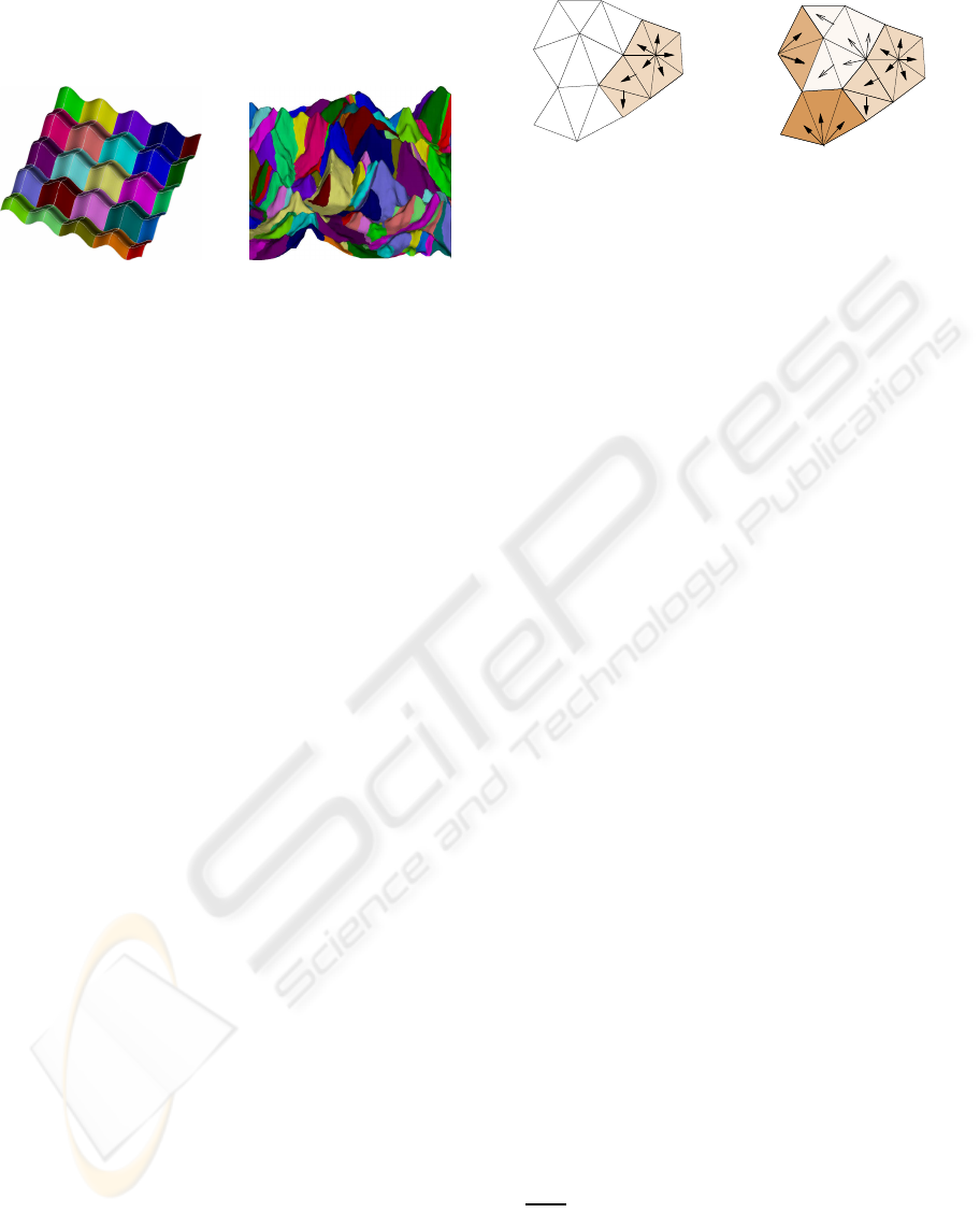
of this decomposition is shown in Figure 5 (a) for a

synthetic function and in Figure (b) for a real data set.

The decomposition algorithm described above al-

(a) (b)

Figure 5: In (a), Unstable decompositions of a synthetic

function f(x, y) = sinx+ siny representing the eggs plateau

surface. In (b), 119 unstable components produced by our

decomposition algorithm applied to a triangulation of the

Mount Marcy consisting of 69718 triangles.

lows us to deﬁne a discrete form of the gradient vec-

tor ﬁeld for a scalar ﬁeld f. A discrete (negative)

gradient vector ﬁeld is deﬁned by the following two

functions. A multi-valuedfunction φ which associates

each local maximum v, corresponding to a compo-

nent C(v) of M, with the top cells γ

′

in St(v) , i.e.,

φ(v) = {γ

′

: γ

′

is a top cell in St(v)}.

With each cell γ in C(v) − {∂C(v) ∪ St(v)}, which

has been used in the extension process, we associate

the added cones (γ, w

). Equivalently,the vertices (w

)

are sufﬁcient to characterize this single-valued func-

tion which we denote by ψ. We have ψ((γ, w

)) =

}. Functions φ and ψ deﬁne the discrete (nega-

tive) gradient vector ﬁeld of f. As in the differen-

tiable case, it denotes the directions in which the func-

tion decreases, and characterizes the critical cells and

points. To obtain a geometric representation of func-

tions φ and ψ, we draw vectors from the initial vertex

v, to all top cells in St(v), and a vector from γ to the

cones (γ, w

) used in the decomposition process. We

obtain a collection of vectors that indicate the direc-

tions in which the scalar ﬁeld is decreasing (cf., Fig-

ures 6).

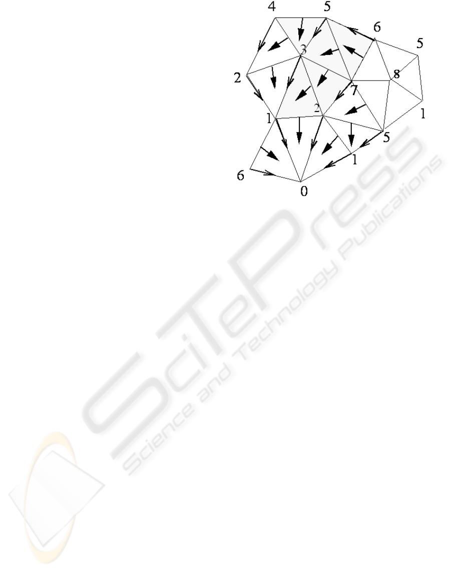
Referring to the example in Figure 6(a), we con-

sider the vertices at which the scalar ﬁeld reaches its

maximum, which is equal to 8. We show the process

of growing the component. The shaded regions in

Figure 6(a) is the component associated with value

8. In Figure 6(b), we show the ﬁnal decomposition

of the complex in 6(a) with its gradient vector ﬁeld.

Each shaded region correspond to an unstable Smale

component.

(a)

(b)

Figure 6: In (a), the decomposition process of K: compo-

nent corresponding to the vertex with the ﬁeld value equal

to 8 with its discrete gradient vector ﬁeld. In (b), the ﬁ-

nal components decomposing K and their discrete gradient

vector ﬁeld.

6 EXTENDED GRADIENT FIELD

AND COMPATIBILITY WITH

FORMAN THEORY

In this Section, we prove that the discrete gradient

ﬁeld obtained from our Smale-like decomposition of

a manifold M endowed with a scalar ﬁeld f can be

extended so that a Forman function F is deﬁned over

M. From this point of view, the scalar ﬁeld f becomes

the restriction of F over the vertices of M, its gradient

vector ﬁeld Grad f becomes a subﬁeld of the gradient

vector ﬁeld of F and the critical points of f are a sub-

set of critical cells of F.

In the construction process of the Smale-like decom-

position seen in Section 5, the expansion of compo-

nents C(v) begins by attaching to St(v), where v is a

local maximum, other cones (γ, w) where γ is a top

simplex in Lk(v) and f(w) is less than all values of

f over vertices of γ. Then function ψ associates, the

(n−1)-simplex, γ with vertex w. For each pair (γ, w),

function ψ can be extended, to a function

ψ, over all

faces σ

of γ, with i = 0 to dim(γ)−1 = n−2 by asso-

ciating σ

with vertex w. Geometric equivalent exten-

sion consists of emanating vectors from all faces of γ

towards vertex w. This is compatible with our decom-

position process since f(w) < f(w

′

) for all vertices w

′

of γ, see Figure 7 below. Note that, according to this

construction, all faces of γ are not critical since they

are tails of vectors. Since a simplex cannot be the

tail and the end of a vector at the same time, then if

a simplex γ

′

= (σ

(n−2)

, w) is used to expand ∂C(v) in

the Smale-like decomposition process, the vector cor-

responding to

ψ(σ

n−2

) has to be removed. This al-

ready characterizes a Forman function over all faces

C(v) − St(v).

Thus, the extended function

ψ can be explicitly de-

ﬁned by

• if γ is a (n − 1)-simplex expanding C(v) then

ψ(γ) := ψ(γ) = {w}, such that (γ, w) expands

MORPHOLOGY-BASED REPRESENTATIONS OF DISCRETE SCALAR FIELDS

141

C(v).

• For all i-simplexes σ

∈ γ, with i = 0, . . ., n− 3 we

set

ψ(σ

) := {w} if

ψ(σ

) has not been deﬁned

before when another (n− 1)-simplex γ incident is

was considered. Otherwise, σ

is skipped since

it has already an attached value by

• For i = n−2 and such that (σ

n−2

, w) does not par-

ticipate to the expansion process of C(v), we have

ψ(σ

n−2

) = {w}.

• Otherwise

ψ(σ

n−2

) =

0. In this case,

cone (σ

n−2

, w) represents a new ex-

panding (n − 1)-simplex of C(v) and

ψ((σ

n−2

, w)) = ψ((σ

n−2

, w)). Then we re-

turn to the ﬁrst point to deﬁne

ψ over faces of

(σ

n−2

, w).

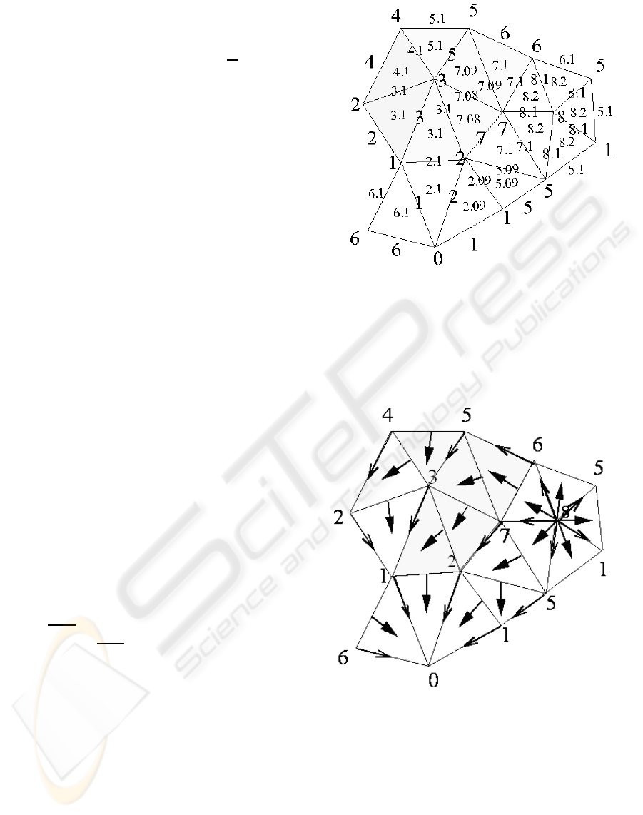
For simplicity, we present in Figure 7 the extended

gradient vector ﬁeld for a 2-dimensional scalar ﬁeld.

Simplexes γ are edges and their faces σ

are vertices

(i.e., we have only i = 0). Vectors emanating from

vertices towards edges are added if the edges do not

participate in the expansion process of the compo-

nent construction. For example, segment γ = [6;7]

expands C(8) by adding triangle ∆ labeled as 6, 7 and

5. Function ψ associates segment [6;7] with vertex

{5}. An arrow from [6;7] towards {5} is drawn. End

points of segment [6;7] are the (n− 2)-simplexes de-

scribed above. Cone (i.e., segment)(6, 5) does not

participate in the expansion of the new component

C(v) := C(v) ∪ ∆. Thus, function

ψ(6) = {5} and a

vector emanating from {6} towards {5} is added to

edge [6;5]. The other vertex {7} of segment [6;7],

with vertex 5 forms an edge that expands the updated

C(v), then

ψ(7) =

0 and no vector is emanating from

{7} towards {5} is drawn in triangle ∆. Note that

the same vertex {7} is revisited again when trian-

gle (7;3;2) is considered. Function

ψ associates {7}

with {2} since edge [7;2] does not expand C(v). Ver-

tex {7} is revisited again a last time when triangle

(7;5;2) is considered. The process skips here ver-

tex {7} since it has already a non-empty value by

ψ.

We see clearly that each simplex in the triangulation

emanates or receives at most one vector. Hence, the

extended gradient vector ﬁeld is a Forman gradient.

Critical cells are those which are not the tail nor the

end of vectors. We have here only one (global) min-

imum {0} and the entire star St(8) as a singular cell

corresponding to the maximal value 8.

In the general case, function F is not uniaue and can

be deﬁned in many ways. In the following, we present

an explicit construction of F. Let γ be a (n − 1)-

simplex expanding a component C(v) to C(v) ∪ {w}

and let σ

be a face of γ where i ∈ {1, . . . , n−1}. Sup-

pose that γ and its faces are visited for the ﬁrst time.

Figure 7: Illustration of the extended gradient vector ﬁeld

for a 2-dimensional scalar ﬁeld. The extension here acts

only on vertices. Arrows are added to edges that do not

participate to the expansion process of componentC(v) with

f(v) = 8.

1. We set F(γ) := max{ f(v

′

) : v

′

is a vertex of γ} +

(n−1)ε, where ε is positive numberchosen so that

F(γ) < f(v). Then we deﬁne F(γ,w) := F(γ).

For faces (σ

)

n−2

i=0

, we set F(σ

) := max{ f(v

′

) :

′

is a vertex of σ

} + iε, for all i ∈ {1, . . . , n− 1}.

Note that for i = 0, simplexes σ

are simply ver-

tices of γ for which we have F(σ

) = f(σ

Let σ

be a face of another simplex σ

⊂

γ (i.e., i < j), then vertices of σ

are in-

cluded in the set of vertices of σ

. Hence

max{ f(v

′

) : v

′

is a vertex of σ

} ≤ max{ f(v

′

) :

′

is a vertex of σ

} and consequently F(σ

) <

F(σ

). This implies that faces of γ are set to be

critical at this deﬁnition step except γ from which

an arrow in emanated towards cone (γ,w).

2. For cones (σ

, w), we deﬁne F((σ

, w)) := F(σ

for all i ∈ {0, 1, . . ., n − 2}. This means that

from each face σ

we emanate an arrow towards

cone (σ

, w) This deﬁnition ensures that Forman

relations (1) and (2) are satisﬁed.

3. Now, for the expansion process of the up-

dated component C(v), (n− 1)-simplexes of type

(σ

n−2

, w) are considered. Let update γ to be equal

to (σ

n−2

, w). At this moment, γ and each of its

faces adjacent to w receive an arrow from a face

of σ

n−2

. We update then w to be the new added

point. Since γ is expanding component C(v) to

a new cone (γ, w), then new arrows will be em-

GRAPP 2007 - International Conference on Computer Graphics Theory and Applications

142

anated from faces of γ towards w. Hence, values

of faces of γ by F should be re-initialized to make

them, ﬁrst, critical in C(v). To do that, we up-

date, ﬁrst, value of ε to be equal ε −

and then

we return to step (1.). Value of ε is updated for

the following reason. Simplex γ is adjacent to two

n− simplexes, the old cone (γ, w) ⊂ C(v) and the

new cone (γ, w) expanding C(v). Then, to pre-

serve Forman relations (1) and (2), value of γ by

F should be less then the value of the old cone

(γ, w).

Step (1.) deﬁnes F over (γ, w), γ and all its

faces. Values of vertices (i.e., 0-simplexes) are

preserved. We return, then to step (2.) to deﬁne

F over all faces of type (σ

, w). New arrows are

hence drawn from faces σ

to (σ

, w) and we go so

on. If a face is re-visited from another expanding

simplex then we assign to the simplex a value that

preserves Forman relations (1) and (2).

By a such construction Forman relations are satisﬁed

over all the simplexes of the complex.

The simplest way to extend f over St(v) is to con-

sider that all simplexes in the interior of St(v) are crit-

ical for F since they are the immediate neighbors of

v which is critical for f. We can deﬁne F for an i-

dimensional face α

of St(v) to be f(v)+iε. Relations

(3) are, thus, satisﬁed over all simplexes of St(v).

In Figure 8, we give an example of construction of

a Forman function that extends the scalar ﬁeld f de-

scribed in Figure 7 with value ε = 0.1. The extended

function preserves Forman relations (1) and (2) and

corresponds to the above formulas deﬁning F. Thus,

the function obtained in the example is a Forman

function.

Function

φ describing the gradient vector ﬁeld over

St(v) can be associated with the restriction of F over

St(v) and function

ψ describing the gradient vector

ﬁeld over

C(v) − St(v) can be associated with the re-

striction of F over C(v) − St(v).

Outside St(v), the extended gradient vector ﬁeld fol-

lows, naturally, the decreasing growth of the function

f over the triangulation simplexes.

To keep the differentiability simulation of the ex-

tended gradient vector ﬁeld over the entire domain,

we keep the geometric representation (by vectors) of

function φ over stars {St(v)} of local maxima {v}.

In order to be consistent with the extension

ψ of ψ

over proper faces of simplexes γ, we extend func-

tion φ, to a function

φ over all simplexes in St(v) by

emanating vectors from v towards all simplexes in-

cident to v. The extended function

φ is deﬁned by

φ(v) = {γ

′

: γ

′

is a simplex in St(v)}.

In Figure 9, we show the representation of both

φ and

Figure 8: Deﬁnition of a Forman function that extends the

scalar ﬁeld over all simplexes and that corresponds to the

extended gradient vector ﬁeld described in Figures 7 and 9

with value ε = 0.1.

ψ for the same scalar ﬁeld represented in Figure7.

Figure 9: General representation of the extended gradient

vector ﬁeld for a 2-dimensional scalar ﬁeld over all the tri-

angulated domain.

7 CONCLUDING REMARKS

Here, we have presented an extended form of a dis-

crete gradient vector ﬁeld associated with a Smale-

like decomposition in order to deﬁne a Forman func-

tion compatible with the decomposition. A Smale-

MORPHOLOGY-BASED REPRESENTATIONS OF DISCRETE SCALAR FIELDS

143

like decomposition simulates well the differentiable

case. Thus, we obtain a good representative of a dis-

crete gradient ﬁeld that combines properties of both

smooth Morse and discrete Forman theories. In our

future work, we are planning to implement processes

for two- and three-dimensional scalar ﬁelds in order

to apply them on real image processing data bases.

We will apply the Forman simpliﬁcation meshes and

its compression process to our extended gradient ﬁeld

in order to deﬁne multi-resolution approach based on

both Morse and Forman theory.

Since the algorithm is dimension-independent, a fur-

ther developmentof this work consists of applying the

approach for clustering .

ACKNOWLEDGEMENTS

This work has been partially supported by a grant of

the Polytechnic University of Valencia, Spain (”Pro-

grama de Apoyo a la Investigacion y Desarrollo

2006”) and by the National Science Foundation un-

der grant CCF-0541032, by the MIUR-FIRB project

SHALOM under contract number RBIN04HWR8, by

the MIUR-PRIN project on ”Multi-resolution model-

ing of scalar ﬁelds and digital shapes” and by the Eu-

ropean Network of Excellence AIM@SHAPE under

contract number 506766.

REFERENCES

Agoston, M. (1976). Algebraic Topology, A First Course,.

Pure and Applied Mathematics, Marcel Dekker.

Bajaj, C. L., Pascucci, V., and Shikore, D. R. (1998). Visu-

alization of scalar topology for structural enhacement.

In Proceedings of the IEEE Conference on Visualiza-

tion ’98 1998, pages 51–58.

Bajaj, C. L. and Shikore, D. R. (1998). Topology preserv-

ing data simpliﬁcation with error bounds. Journal on

Computers and Graphics, 22(1):3–12.

Danovaro, E., De Floriani, L., and Mesmoudi, M. M.

(2003). Topological analysis and characterization of

discrete scalar ﬁelds. In Asano, T., Klette, R., and

Ronse, C., editors, Theoretical Foundations of Com-

puter Vision, Geometry, Morphology, and Computa-

tional Imaging, volume 2616 of Lecture Notes on

Computer Science, pages 386–402. Springer Verlag.

DeFloriani, L., Mesmoudi, M. M., and Danovaro, E.

(2002a). Extraction of Critical Points and Nets Based

on Discrete Scalar Fields. In To appear In Proceed. of

Eurographics conference.

DeFloriani, L., Mesmoudi, M. M., and Danovaro, E.

(2002b). Smale-like Decomposition for Discrete

Scalar Fields. In To appear In Proceed. of Inter. Conf.

on Pattern Recognition.

Edelsbrunner, H., Harer, J., and Zomorodian, A. (2001).

Hierarchical morse complexes for piecewise linear 2-

manifolds. In Proc 17th Sympos. Comput. Geom.,

pages 70–79.

Forman, R. (1998). Morse Theory for Cell Complexes. Ad-

vances in Mathematics, 134:90–145.

J.Toriwaki and Fukumura, T. (1975). Extraction of struc-

tural information from grey pictures. Computer

Graphics and Image Processing, 7:30–51.

Lewiner, T., Lopes, H., and Tavares, G. (2002a). Opti-

mal discrete morse functions for 2-manifolds. Techni-

cal report, Pontiﬁcia Universidade Catolica do Rio de

Janero.

Lewiner, T., Lopes, H., and Tavares, G. (2002b). Visualiz-

ing forman’s discrete vector ﬁeld. In H.-C. Hege, K.

P. E., editor, to appear in Proceed. of Mathematical

Visualization III, Springer.

Milnor, J. (1963). Morse Theory. Princeton University

Press.

Nackman, L. R. (1984). Two-dimensional critical point

conﬁguration graph. IEEE Transactions on Pattern

Analysisand Machine Intelligence, PAMI-6(4):442–

450.

Peucker, T. K. and Douglas, E. G. (1975). Detection of

surface-speciﬁc points by local paprallel processing

of discrete terrain elevation data. Graphics Image

Processing, 4:475–387.

Smale, S. (1960). Morse inequalities for a dynamical

system. Bulletin of American Mathematical Society,

66:43–49.

Thom, R. (1949). Sur une partition en cellule associ´ees a

une fonction sur une vari´et´e. C.R.A.S., 228:973–975.

Watson, L. T., Laffey, T. J., and Haralick, R. (1985). Topo-

graphic classiﬁcation of digital image intensity sur-

faces using generalised splines and the discrete cosine

transformation. Computer Vision, Graphics and Im-

age Processing, 29:143–167.

GRAPP 2007 - International Conference on Computer Graphics Theory and Applications

144