LOCAL MULTIRESOLUTION OF A MESH
BASED ON
3
SUBDIVISION AND SURFACE
DISCONTINUITIES
Olivier Guillot and Jean-Paul Gourret
Laboratoire Informatique, Image, Interaction (L3i)
Université de La RochelleIUT, Department d’Informatique
15 Rue François de Vaux de Foletier 17026 La Rochelle Cedex, France
Keywords: Mesh, surface discontinuities, local multiresolution, analysis, synthesis, compression ratio.
Abstract: We build a local multiresolution of meshes when the connectivity is resulting from an enhanced
3
subdivision of a coarse mesh template. We use the concept of biorthogonality and lifting to develop a
set of filters for local analysis and local synthesis. The enhanced
3
subdivision, we developed, takes into
account natural surface discontinuities during the subdivision process. The multiresolution based on our
enhanced
3
subdivision permits to obtain a great compression ratio.
1 INTRODUCTION
A project of surface meshing for still and animated
images and associated software has been developed
at L3i for several years. Our goal is to build a
multiresolution analysis to compress mesh
information in order to permit fast transmission of
shapes on networks and to allow fast visualization
via levels of details. We use wavelet theory. The
wavelet functions are deduced from scaling
functions based on subdivisions.
There are two main categories of subdivision
schemes: the subdivision inserting vertices on edges
and the subdivision inserting vertices on faces. Each
one of these can use an approximation method or an
interpolation method. Among all the approximation
methods for subdivisions inserting vertices on edges,
we can cite (Doo et al. 1978), (Catmull and Clark
1978) and (Loop 1987). Among interpolation
methods for subdivisions inserting vertices on edges
the method of (Halstead et al. 1993) is a modified
Catmull-Clark subdivision. The most famous one is
the “butterfly” method (Dyn et al. 1990), which
gives a G1 continuity of the limit surface, with a
minimal number of neighbors and whatever the
connectivity of the vertices. A modified butterfly
method which ensures a better continuity has been
proposed by (Dyn et al. 1993) and (Zorin et al.
1996). Among approximation methods for
subdivisions inserting vertices on faces, we can cite
the
3
subdivision of Kobbelt (Kobbelt 2000).
Among interpolation methods, we can cite the
3
Subdivision of Labsik and Greiner (Labsik and
Greiner 2000). All these subdivision methods do not
take into account the natural discontinuities of the
surface.
Subdivision of meshes with natural surface
discontinuities has been studied by (Hoppe et al.
1994). The study is focused on subdivision inserting
vertices on edges and does not include a
multiresolution analysis.
The basic principles of multiresolution analysis and
wavelets were given by (Meyer 1986), (Meyer 1988)
for mathematical aspects, by (Mallat 1989) for
signals and images and by (Lounsbery et al. 1997)
and (Schröder and Sweldens 1995) for surfaces.
Schröder and Lounsbery worked on subdivision
inserting vertices on edges for meshes without
natural surface discontinuities.
A subdivision allows synthesizing a shape. It
increases the resolution of a coarse mesh, called
“control mesh”, and converges on a limit surface. A
multiresolution analysis permits to decrease the
resolution of a fine mesh without lost of information.
In the case of a subdivided mesh, the synthesis is
simply the subdivision of the coarse mesh and the
analysis consists in rebuilding the coarse mesh from
180
Guillot O. and Gourret J. (2007).
LOCAL MULTIRESOLUTION OF A MESH BASED ON â
´
LŽ3 SUBDIVISION AND SURFACE DISCONTINUITIES.
In Proceedings of the Second International Conference on Computer Graphics Theory and Applications - GM/R, pages 180-187
DOI: 10.5220/0002081701800187
Copyright
c
SciTePress

the subdivided mesh. In the case of a complex mesh
that is not the result of a subdivision but has the
connectivity of a subdivided mesh, the analysis
provides a low-resolution approximation mesh.
There exists remeshing methods to obtain this kind
of mesh (Eck et al. 1995), (Lee et al. 1998). In order
to rebuild the original mesh by the synthesis of the
low-resolution mesh, the analysis computes and
store errors, called details, at every level.
The multiresolution theory assures us that the
analyzed mesh is the best approximation of the
original mesh at this level for the chosen dot
product.
Because the subdivision tends to a smooth limit
surface, the analysis of a mesh representing a
smooth limit surface generates many null details.
That’s why the analysed version of a mesh and the
non null details can be stored more efficiently than
the original mesh.
In this paper we introduce a multiresolution analysis
of meshes when the connectivity is resulting from an
enhanced
3
subdivision taking into account
discontinuities. We choose a subdivision inserting
vertices on faces because the meshes are growing
slower than methods by insertion of vertices on
edges. We enhanced the original
3
subdivision of
Labsik and Greiner to take into account the natural
discontinuities of a surface, such as darts, creases
and boundaries (Guillot and Gourret 2006a) (Guillot
and Gourret 2006b). Having this subdivision
scheme, we build a multiresolution analysis, which
handles discontinuities. Moreover, due to the high
amount of data in recent meshes, we develop a local
analysis, i.e. the calculation should include only a
part of the data at a time.
The multiresolution analysis developed in this paper
works with every subdivision scheme. An analogous
approach is done by (Olsen et al. 2005). Their
calculation starts from a very small neighbourhood
which is recursively enhanced by a method similar
to the lifting scheme. So, the size of filter is growing
until an optimization of the magnitude of details is
reached. We build our wavelets with only one lifting
scheme. Then a recursive approach constrains the
number of null details. Moreover our method uses
natural discontinuities to minimize magnitude of
details.
In section 2, we present the principles of a global
multiresolution and some definitions. In section 3,
we explain how to process the local calculus of
scaling and wavelet functions using biorthogonality
and lifting scheme. In Section 4 we describe how to
perform locally a synthesis and in section 5 we
describe how to perform locally an analysis. Section
6 is dedicated to results, and section 7 is dedicated to
conclusion and future works.
2 MULTIRESOLUTION
ANALYSIS BASED ON
SUBDIVISION
2.1 Our Enhanced
3
Subdivision
The enhanced
3
subdivision is based on the
insertion of a new vertex in each triangular face. We
start from a control mesh at subdivision level j=0. A
vertex is inserted in each face. Then new faces are
created joining the new vertices to the initial vertices
and to the new vertices in immediate
neighbourhood.
Doing this, a new vertex always shares 6 faces.
The mesh resulting from one subdivision of level j is
called the level j+1.
A mesh M
j
of level j has n
j
vertices and f
j
faces. We
call Y
j
the set of vertices in the mesh of level j and
K
j
its connectivity, so M
j
= (K
j
, Y
j
) represent the
level j.
A direct property is that
n
j+1
– n
j
= f
j
= 3.f
j-1
= …= 3
j
.f
0
Far of natural surface discontinuities and far of
extraordinary vertices (non 6 connected vertices),
our enhanced
3
subdivision uses the method of
Labsik-Greiner or of Kobbelt (for accuracy we
introduce the name Labsik-Greiner formula and
Kobbelt formula in this paper). Otherwise we
developed a formulation explained in (Guillot and
Gourret 2006b).
2.2 Multiresolution Analysis
Generally a mesh M is obtained from a cloud of
points acquired by a 3D scanner. So the number of
vertices and the connectivity are not the result of
recursive subdivisions (K ≠ K
j
). Our multiresolution
analysis method needs that the connectivity of the
starting high level mesh is the result of a recursive
subdivision (K = K
j
). We suppose that K = K
j
in
what follows. It means for example that most of the
vertices are 6-connected and that extraordinary
vertices, of connectivity different of 6, are
sufficiently spaced. Note that as said in section 2.1, a
new vertex always shares 6 faces: it is always of
LOCAL MULTIRESOLUTION OF A MESH BASED ON v3 SUBDIVISION AND SURFACE DISCONTINUITIES
181
connectivity 6, so the extraordinary vertices are not
introduced by the subdvisivion process. They are
defined in the control mesh M
0
and they remain
through the recursive subdivisions.
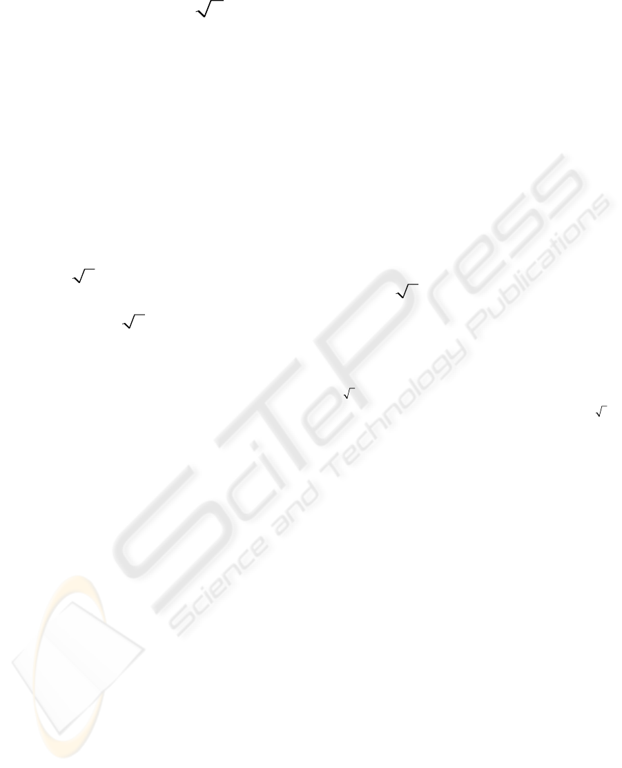
Figure 1: Analysis from level 2 to level 0.
The analysis of a level j+2, builds a level j+1 and a
set of details called Z
j+1
. Recursively the level j+1
can be analysed as a level j and a set of details Z
j
.
Let’s call A
j
the matrix that transform Y
j+1
into Y
j
and B
j
the matrix that transform Y
j+1
into Z
j
.
The detail Z
j+1
has exactly three times more vertices
than Z
j
. We show in Figure 1 the analysis from level
2 to level 0.
Let’s call Y
j
(n) the n
th
vertex of Y
j
. The details Z
j
are
considered as a list of virtual points (points not
connected via K
j
).
In what follows V
i
is the i
th
vertex of Y
j
, V’
i
is the i
th
vertex of Y
j+1
and W
i
is the (i - n
j
)
th
vertex of Z
j
.
2.3 Multiresolution Synthesis
The synthesis is the reconstruction of the level j+1
from the level j and the details Z
j
. A second
synthesis rebuilds the level j+2 from the level j+1
rebuilt and from the details Z
j+1
. Thus the level j+2
can be obtained from the level j and the details Z
j
and Z
j+1
.
Figure 2: Synthesis from level 0 to level 2.
Let’s call P
j
the matrix that subdivide Y
j
and call Q
j
the matrix that uses the details Z
j
. The action of Q
j
on Z
j
gives the difference between Y
j+1
and the
subdivision of Y
j
. We show in Figure 2 the synthesis
from level 0 to level 2.
3 LOCAL COMPUTATION OF
SCALING AND WAVELET
FUNCTIONS
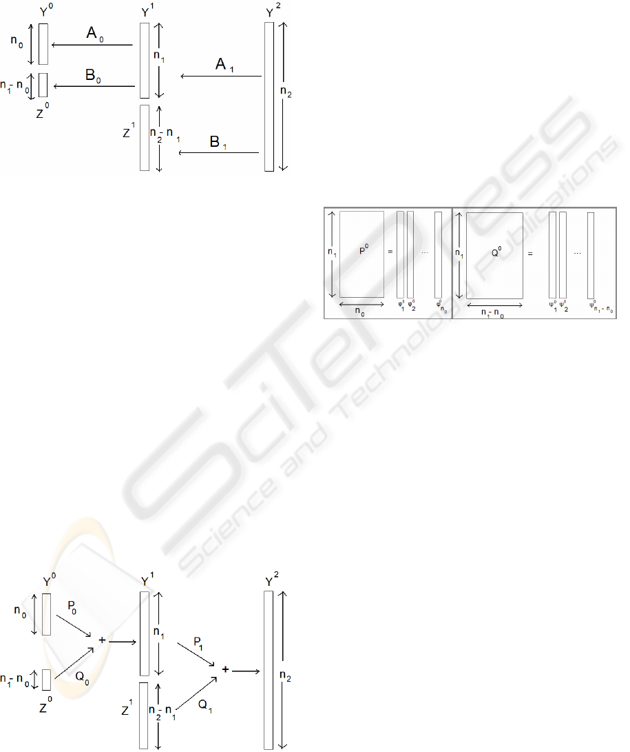
In order to build a multiresolution, we need a scaling
function φ and a wavelet function ψ. They define the
global matrices P
j
and Q
j
as shown in Figure 3. We
never compute the whole P
j
or Q
j
matrices, only
rows or columns of these matrices.
Figure 3: Definition of the global matrices P
0
and Q
0
.
3.1 Local Computation of φ
j
Note that “local computation of φ
j
” means that the
computation itself is local, not the function φ
j
. Let’s
V’
i
be a vertex in Y
j+1
and D’
i
be the d-disk in Y
j+1
centred on V’
i
. The d-disk centered on V’
i
is the set
of vertices connected to V’
i
by less than d edges.
In what follows, we will suppose that every
calculation is local around a vertex, which means
that to synthesize a vertex V’
i
in Y
j+1
, we need to
consider some vertices in Y
j
and some points in Z
j
.
The vertices of Y
j
and the points of Z
j
are in
D
i
= {V
i
; V’
i
є D’
i
} U { W
i
; W’
i
є D’
i
}.
If i is in [1,n
j
], φ
j
i
represents the influence of the
vertex V
i
in the computation of the new vertices in a
one level subdivision, it is the scaling function
associated with V
i
. The influence of the vertex V
i
is
local, so we can compute it locally, in fact V
i
only
influences the vertices of D’
i
.
The scaling function φ
j
i
depends on the connectivity
of the vertices around D’
i
.
For example, when we use the Labsik-Greiner
interpolation formula with twelve neighbours
(Figure 4) the disk D’
i
is shown in Figure 5. Note
that because the Labsik-Greiner formula is an
interpolation method only black vertices are
GRAPP 2007 - International Conference on Computer Graphics Theory and Applications
182
influenced by V
i
, white vertices are not influenced
by V
i
.
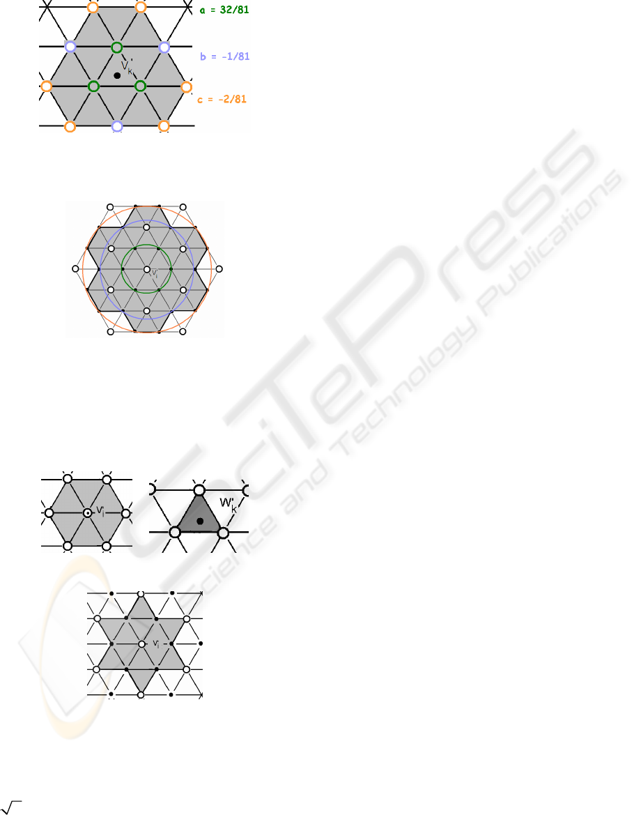
Figure 4: Stencil of Labsik-Greiner formula (the twelve
circled neighbours are weighted a, b or c to calculate the
black vertex V’
k
).
Figure 5: 3-Disk D’
i
for Labsik-Greiner formula (V
i
influences black vertices, with a, b, c weights).
For example, when we use Kobbelt formula (Figure
6), D’
i
is the 2-disk shown in Figure 7. Note that
because Kobbelt is an approximation method, black
and white vertices are influenced by V
i
.
Figure 6: Stencils for kobbelt formula.
Figure 7: D’
i
for the Kobbelt formula.
D’
i
depends on the method of subdivision and on the
proximity or not of natural discontinuities or
extraordinary vertices. See (Guillot and Gourret
2006b) for more explanations on the enhanced
3
subdivision. Calculations are now implemented
in our software MEFP3C (Khamlichi and Gourret
2004). Note that taking discontinuities into account
enlarges the size of D’
i
.
For every V’
k
in Y
j+1
, we note φ
j
i
(k) the influence of
V
i
on the computation of V’
k
. If V’
k
is not in D’
i
, V
i
has no influence, so φ
j
i
(k) = 0. If V’
k
is in D’
i
, φ
j
i
(k)
can be obtained by simulating the calculation of V’
k
in the subdivision algorithm, we obtain the weight of
V
i
in the stencil around V’
k
.
3.2 Local Computation of ψ
j
Note that “local computation of ψ
j
” means that the
computation itself is local, not the function ψ
j
. For k
in [1 , n
j+1
- n
j
] ψ
j
k
is the wavelet function associated
with W
k
(W
k
= Z
j
(k - n
j
)).
Knowing the φ
j
function, we should build the ψ
j
function using the global orthogonal condition
between φ
j
and ψ
j
:
For all i in [1,n
j
], for all k in [1 , n
j+1
- n
j
]
< φ
j
i
, ψ
j
k
> = 0.
But a global computation is too expensive. So we
release this constraint to something local.
We use the concept of biorthogonality with lazy
wavelet (Sweldens 1996). For ψ
lazy k
we choose the
dirac δk. Let’s V
a
, V
b
and V
c
be the vertices of the
face of Y
j
in which we insert W’
k
. Our lifting
operation to enhance the orthogonality of the lazy
wavelets consists in writing :
ψ
j
k
= ψ
j
lazy k
+ α. φ
j
a
+ β. φ
j
b
+ γ. φ
j
c
, where α, β, γ are
real numbers that we compute for every k and every
j writing the system :
< φ
j
a
, ψ
j
k
> = 0
< φ
j
b
, ψ
j
k
> = 0
< φ
j
c
, ψ
j
k
> = 0
It is a 3x3 system, easily solved, done for every k.
φ
j
a
is known by its values on every vertex of Y
j+1
so
it can be seen as a vector of R
nj+1
. Let’s consider ψ
j
k
as a vector of R
nj+1
. To calculate < φ
j
a
, ψ
j
k
> we use
the Euclidean inner product of φ
j
a
and ψ
j
k
as vectors
of R
nj+1
. We do not use the usual inner product first
defined by Lounsbery.
Our wavelet function is the sum of three scaling
functions. Thus we can compute locally ψ
j
k
. An
example for the regular case of the Labsik-Greiner
formula is shown in Figure 8.
LOCAL MULTIRESOLUTION OF A MESH BASED ON v3 SUBDIVISION AND SURFACE DISCONTINUITIES
183
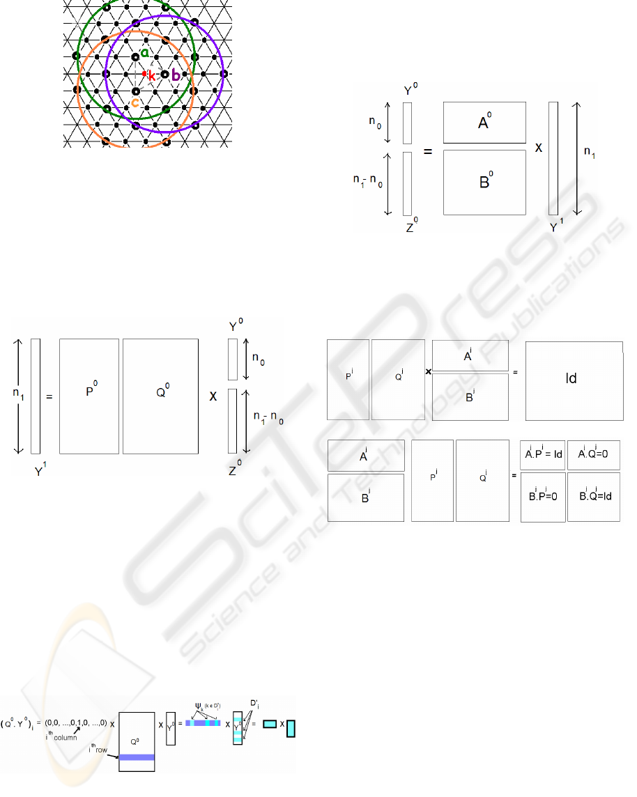
Figure 8: 4-Disk D’
k
of the wavelet function ψ
j
k
associated
with the Labsik-Greiner formula.
4 LOCAL SYNTHESIS
The synthesis is the sum of the result of the P
j
and Q
j
matrices applied to Y
j
. The synthesis is computed
with the matrices P
j
and Q
j
as show in Figure 9.
Figure 9: Synthesis from level 0 to level 1.
The action of P
j
on Y
j
is exactly the result of the
subdivision which is a local computation, i.e. the
computation of Y
i
j+1
is local around Y
i
j
.
To compute the action of Q
j
on Z
j
, we need the i
th
row of Q
j
. We have already assumed that this row
has only non null factors in the columns representing
the vertices of D’
i
. Let’s W
k
be a point of Z
j
. We
know how to compute ψ
k
j
where only the i
th
coefficient interests us.
The calculation of the i
th
row of Q
j
needs just the
calculation of ψ
k
j
for every W
k
in Z
j
.
Figure 10: Computation scheme of Y
0
i
= Q
0
i
.Y
0
.
5 LOCAL ANALYSIS
The analysis is globally computed with the matrices
A
j
and B
j
as shown in Figure 11.
Figure 11: Analysis from level 1 to level 0.
A
j
and B
j
are usually computed as the inverse of the
global matrix [PQ]
j
whose properties are shown in
Figure 12.
Figure 12: Global matrices.
5.1 Local Analysis: the Built of Y
j
Let’s V
i
be in Y
j
. The i
th
row of A
j
applied on Y
j+1
gives us V
i
.
We assume that the action of A
j
around V
i
can be
computed locally on D’
i
. If A
j
ik
is the term of A
j
on
the i
th
row and the k
th
column, we can assume that
A
j
ik
= 0 if Y
j+1
(k) is not in D’
i
. To compute the result
of the i
th
row of A
j
, we need the (A
j
)
ik
for k verifying
Y
j+1
(k) in D’
i
. In section 3 we saw that we can
compute φ
k
and ψ
k
for every k.
Let’s A
j
i
be the i
th
row of A
j
with only the
coefficients corresponding to a column h that verify
Y
j+1
(h) in D’
i
.
Let’s call (P
j
k
)
kєD’i
the matrix containing the P
j
k
where k is in D’
i
. It is also the matrix containing the
φ
k
j
when Y
j+1
(k) in D’
i
, with just the rows of number
h verifying Y
j+1
(h) in D’
i
.
GRAPP 2007 - International Conference on Computer Graphics Theory and Applications
184
From the equation A
j
.P
j
= Id we have just kept some
rows and some columns so we can write the
following equation:
A
j
i
.(P
j
k
)
kєD’i
= (0, 0, 0, …, 1, 0, 0, …, 0)
The one is placed as i in D’
i
.
In the same way we build (Q
j
k
)
kєD’i
as the matrix
containing the ψ
j
k
when Y
j+1
(k) is in D’
i
with just the
rows of number h when Y
j+1
(h) is in D’
i
. The
equation A
j
.Q
j
= 0 gives
A
j
i
.(Q
j
k
)
kєD’i
= (0, …, 0) .
The matrix [(P
j
k
)
kєD’i
, (Q
j
k
)
kєD’i
] is a square matrix (of
size given by the number of vertices in D’
i
). We
compute A
j
i
with the inverse of [(P
j
k
)
kєD’i
, (Q
j
k
)
kєD’i
].
Eventually, V
i
= A
j
i
. Y
j+1
.
5.2 Local Analysis: the Built of Z
j
The i
th
row of B
j
applied on Y
j+1
gives us W
i+nj
.
Let’s use again the matrices B
j
i
, (P
j
k
)
kєD’i
and
(Q
j
k
)
kєD’i
, from the equations:
B
j
.P
j
= 0 and B
j
.Q
j
= Id
we can write:
B
j
i
. (P
j
k
)
kєD’i
= 0 and B
j
i
. (Q
j
k
)
kєD’i
= (0, 0, …, 1, 0,
…,0) with the one placed as i in D’
i
.
By just inverting [(P
j
k
)
kєD’i
, (Q
j
k
)
kєD’i
] we obtain B
j
i
and so W
i
.
6 RESULTS
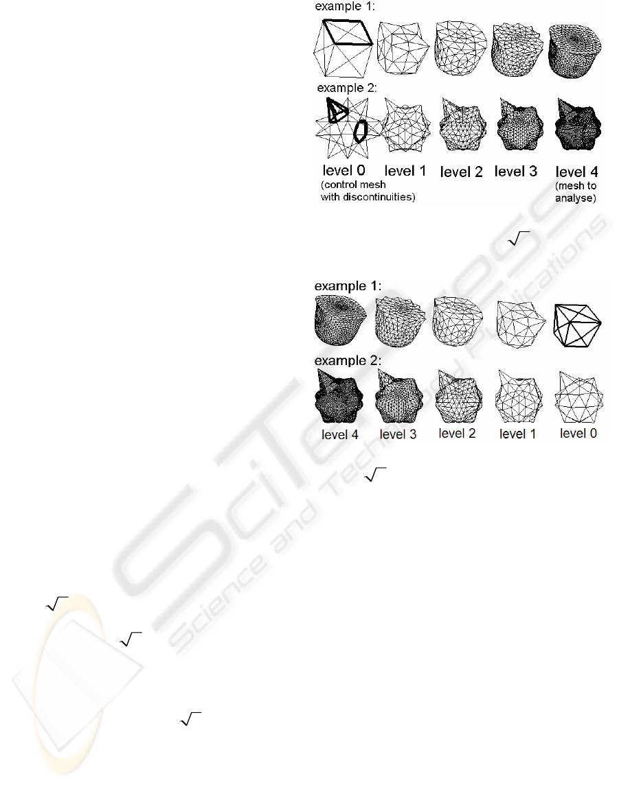
Examples presented are not realistic ones. There are
only given to prove working of our method. We
show in Figure 13, two examples. In order to get
meshes with the connectivity of a subdivided mesh
that are not just the result of a previous subdivision,
we created meshes with discontinuities and we
subdivided them 4 times with our approximation
enhanced
3
subdivision scheme. Then we have
implemented our multiresolution analysis from our
interpolating enhanced
3
subdivision scheme.
The meshes to analyse have the connectivity of
meshes subdivided four times, so we can analyse
them 4 times.
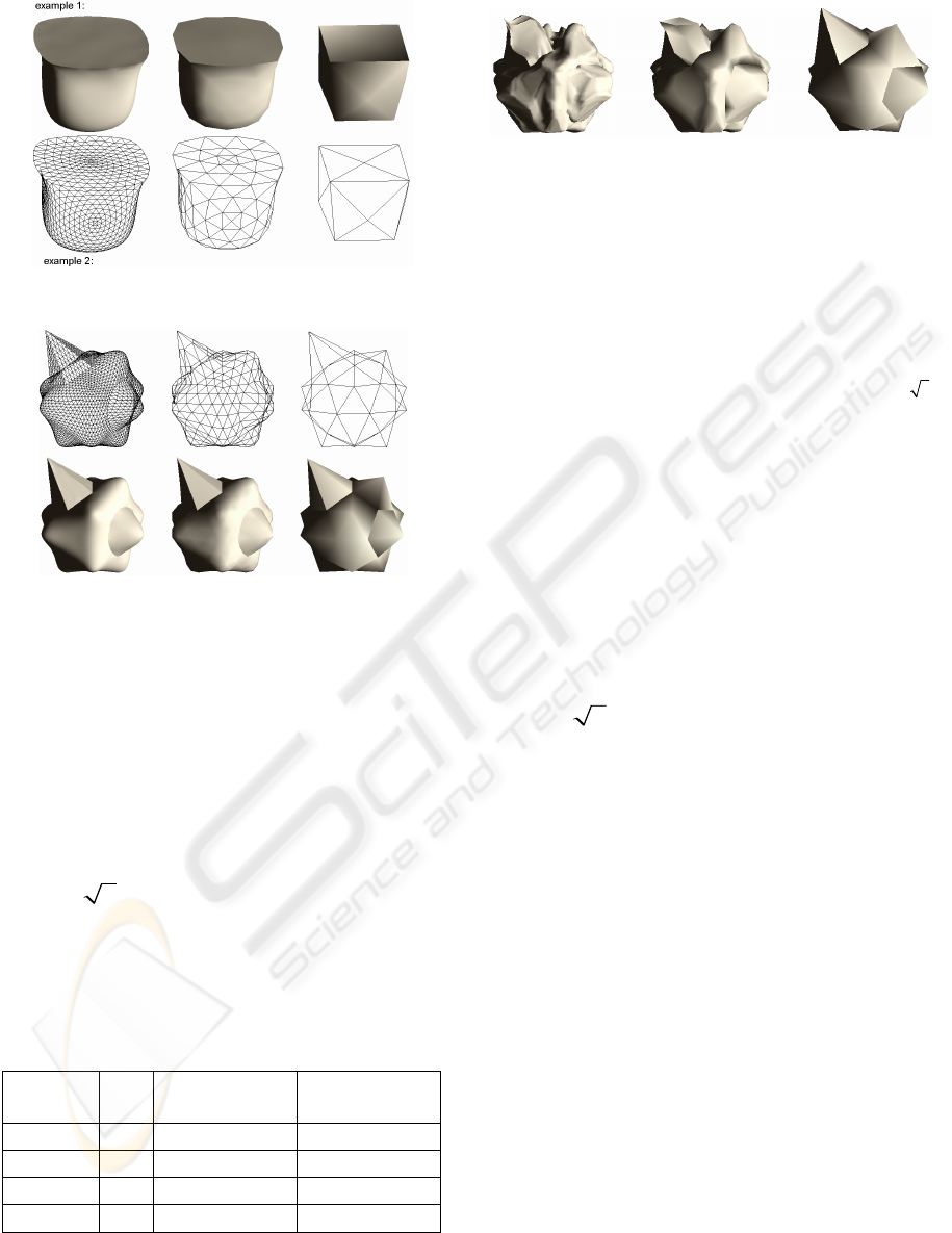
We show in Figure 14 the result of four analyses.
Note that because our enhanced
3
subdivision is
a subdivision inserting vertices on faces, the
discontinuities do not belong to edges of the meshes
of odd level 1 and 3 (Guillot and Gourret 2006b),
only the even level produced by the analysis (level 0
and 2) should be visualized as shown in Figure 15.
Figure 13: The construction of the meshes to analyse
(construction with our enhanced
3
approximation
method).
Figure 14: The result of four analyses with our
enhanced
3
interpolation method.
6.1 Compression
With the mesh of level 0 and the four details Z
0
, Z
1
,
Z
2
and Z
3
, we can rebuild exactly the original mesh.
The size of (Y
4
) is the same as the size of (Y
0
, Z
0
,
Z
1
, Z
2
, Z
3
). Because the subdivision tends to a
smooth limit surface, the analysis of a mesh
representing a smooth limit surface generates many
approximately null details. Considering some of this
details as null do not generate a great difference
between the rebuilt mesh and the original mesh. That
is why the analysed version of a mesh and the non
null details can be stored more efficiently than the
original mesh. We developed a constraint on the
details (not explained in this paper) in order to
ensure that the rebuilt mesh will not differ from the
original mesh by more than a given tolerance
epsilon. It means that for every vertex i, |Y
i
4
original
-
Y
i
4
rebuilt
| ≤ epsilon * diameter of the bounding sphere.
We show in Table 1, the percentage of details kept
because they cannot be considered as null factors for
LOCAL MULTIRESOLUTION OF A MESH BASED ON v3 SUBDIVISION AND SURFACE DISCONTINUITIES
185
the 2 examples. The third column when the analysis
takes into account natural surface discontinuities.
Our multiresolution analysis method based on the
standard Labsik-Greiner formula, modified around
extraordinary vertices, and without natural surface
discontinuities processing permits to obtain a good
compression ratio as shown in the second column of
table 1.
Our multiresolution analysis method based on our
enhanced
3
subdivision, with natural surface
discontinuities, permits us to obtain an even better
compression ratio.
We show in Figure 16 a third example, which is the
second example at level 4, deformed by MEFP3C.
Table 1: Compression ratio in order to archive a precision
of ε.
є without
discontinuities
with
discontinuities
Example 1 1% 81% 87%
Example 2 1% 81% 88%
Example 2 1‰ 59% 63%
Example 3 1% 65% 65%
7 CONCLUSION AND FUTURE
WORK
The local multiresolution analysis of meshes
presented in this paper uses our enhanced
3
subdivision. Because the calculations are local, the
algorithm could be parallelized on multiprocessor
computers.
Without discontinuities, the disk D’
i
to synthesize a
vertex V’
i
is a 3-disk for the scaling function and a
4-disk for the wavelet function. Because our
software deduces ψ from φ, it is only necessary to
impose the disk size for φ. Without discontinuities,
the disk D’
i
to analyze a vertex V’
i
is a 4-disk. This
result is an experimental result.
The multiresolution analysis developed in this paper
works with every subdivision scheme.
Our multiresolution analysis method based on our
enhanced
3
subdivision which takes into account
natural surface discontinuities permits us to obtain a
great compression ratio.
We are presently working on boundaries that are
handled by our enhanced subdivision but not yet
implemented in our multiresolution analysis and we
are also working on remeshing algorithms. Then we
will be able to process realistic shapes such as faces
and bodies.
ACKNOWLEDGEMENTS
This work was supported by a French region Poitou-
Charentes grant.
REFERENCES
Doo D., (1978) A subdivision algorithm for smoothing
down irregularity shaped polyhedrons. Proc. Int. Tech.
In Comp. Aided Des, pp. 157-165.
Catmull.E, Clark J., (1978) Recursively generated B-
spline surfaces on arbitrary topological meshes. Comp.
Aided Des. pp.350-355.
Figure 15: The meshes to analyse (level 4) and the level 2
and 0 obtained from analysis with discontinuities.
Figure 16: The mesh to analyse (level 4 of example 2
deformed) and the level 2 and 0 obtained from analysis
with discontinuities.
GRAPP 2007 - International Conference on Computer Graphics Theory and Applications
186

Loop C.T., (1987) Smooth subdivision surfaces based on
triangles. Master’s thesis, Dept. Of Mathematics,
Univ. Of Utha.
Halstead M., Kass M., DeRose T., (1993) Efficient fair
interpolation using Catmull-Clark surfaces. Proc.
ACM SIGGRAPH. pp. 35-44.
Dyn N., Levin D., Gregory J.A. (1990) A butterfly
subdivision scheme for surface interpolation with
tension control. ACM Trans. On Graphics, Vol 9(2),
pp.160-169.
Dyn N., Head S., Levin D., (1993) Subdivision schemes
for surface interpolation. Comp. Geometry. pp.97-118.
Zorin D., Schröder P., Sweldens W. (1996) Interpolating
subdivision for meshes with arbitrary topology. Proc.
ACM SIGGRAPH., pp. 189-192.
Kobbelt L. (2000)
3
subdivision. Proc. SIGGRAPH,.
pp.103-112.
Labsik U., Greiner G., (2000) interpolatory
3
subdivision. proc. EUROGRAPHICS. Vol 19(3).pp.?
Hoppe H., DeRose T., Duchamp T., Halstead M., Jin H.,
McDonald J., (1994) Piecewise smooth surface
reconstruction. Conf. Proc. ACM SIGGRAPH. pp.295-
302.
Meyer Y., (1986) Ondelettes et fonctions splines, sem.
Equations aux dérivés partielles, Ecole Polytechnique,
Paris, France.
Meyer Y., (1988) ondelettes et opérateurs, Hermann.
Mallat S., (1989) A theory for multiresolution signal
decomposition : the wavelet representation. IEEE
Trans. On Pattern Analysis and Machine Intelligence.
Vol.11(7), pp. 674-693.
Lounsbery M., DeRose T.D., Warren J., (1997)
Multiresolution analysis for surfaces of arbitrary
topological type ACM Trans.On Graphics. Vol.16(1),
pp.34-73.
Schröder P., Sweldens W., (1995) Spherical wavelets :
Efficiently representing functions on the sphere.
SIGGRAPH’95 Conf. Proc. pp.161-172.
Eck M., DeRose T., Duchamp T., Hoppe H., Lounsberry
M., Stuetzle W., (1995) Multiresolution analysis of
arbitrary meshes, ACM SIGGRAPH ’95, pp.173-182
Lee A., Sweldens W., Schröder P., Cowsar L., Dobkin D.
(1998) MAPS : Multiresolution adaptive
parameterization of surfaces, ACM SIGGRAPH
pp.95-104
Guillot O., Gourret J.P., (2006a) square root 3 subdivision
and 3-connected meshes with creases, boundaries and
holes. In poster session of Journal of WSCG,
Plzen(CZ).
Guillot O., Gourret J.P., (2006b) Subdivisions et
discontinuités pour le maillage des surfaces dans le
système logiciel MEFP3C. Session MB1-3., CNRIUT,
Brest.
Olsen L., Smavati F.F., Bartels R.H., (2005)
Multiresolution B-splinesbased on wavelet constraints
journal Eurographics symposium on geometry
processing, pp.1-10, M. Debrun, H. Pottmann
(editors), 2005
Khamlichi J., Gourret J.P., (2004) MEFP3C : un système
logiciel pour le maillage évolutif de forme avec
pavage par polygone à sommets 3-connexes. CNRIUT
Nice pp.81-88
Sweldens W., (1996) the lifting scheme : a custom
designed construction of biorthogonal wavelets.
Applied and computational analysis, Vol.3(2), pp.186-
200
LOCAL MULTIRESOLUTION OF A MESH BASED ON v3 SUBDIVISION AND SURFACE DISCONTINUITIES
187
