
REALISTIC TRANSMISSION MODEL OF ROUGH SURFACES
Huiying Xu and Yinlong Sun
Department of Computer Sciences, Purdue University, West Lafayette, Indiana 47907, USA
Keywords: Transmission model, BTDF, rough surface, Monte Carlo simulation, light scattering.
Abstract: Transparent and translucent objects involve both light reflection and transmission at surfaces. This paper
develops a realistic transmission model of rough surfaces using the statistical ray method, which is a
physically based approach that has been developed recently. The surface is assumed locally smooth and
statistical techniques can be applied to calculate light transmission through a local illumination area. We
have obtained an analytical expression for single scattering. The analytical model has been compared to our
Monte Carlo simulations as well as to the simulations by others, and good agreements have been achieved.
The presented model has a potential for realistic rendering of transparent and translucent objects.
1 INTRODUCTION
Light scattering by objects is generally characterized
by a bidirectional scattering distribution function
(BSDF) (Glassner, 1995)
(, ,)
(, , , ,)
(, ,)cos
oo o
iioo
iii i i
dL
Ld
θϕλ
ρθ ϕ θ ϕ λ
θϕλ θ
=
Ω
, (1)
which is the ratio of the scattered radiance
o
dL
in
the outgoing direction
(, )
oo
θ
ϕ
to the irradiance
cos
iii
L
d
θ
Ω in the direction (, )
ii
θ
ϕ
(Figure 1) at
wavelength
λ
. When referring to reflection or
transmission, a BSDF becomes a bidirectional
reflectance distribution function (BRDF) or a
bidirectional transmittance distribution function
(BTDF). This paper studies the case of transmission.
In computer graphics application, materials may
be classified into three major types: opaque,
transparent and translucent. An opaque object only
involves reflection, a transparent object involves
both reflection and transmission, and a translucent
object has volumetric scattering in addition to
reflection and transmission at the object surface.
Thus, a transmission model is needed for not only
transparent but also translucent objects. Such objects
include glass wares, plastics, ices, biological tissues,
marbles, waxes, and so on.
There has been extensive research on modelling
BRDFs in computer graphics, but studies on BTDFs
are limited. Different from at an opaque surface, a
scattering process at a surface of some transparent or
translucent material is generally a combination of
reflection and transmission events, and the number
of the events may be one (single scattering), two or
more (multiple scattering). Solving the case of single
scattering is a basis for solving the case of multiple
scattering.
Figure 1: Light scattering at a surface (transmission case).
This paper presents a realistic transmission
model of rough surfaces. The model is derived using
a physically based approach called the statistical ray
method that has been developed recently by Sun
(2007). The key assumption of the surface is that the
surface is sufficiently smooth locally and statistical
techniques can be applied to calculate light
transmission through a local illumination area. We
have obtained an analytical expression for single
scattering. The model has been compared to our
Monte Carlo simulations as well as to the
simulations by others, and good agreements have
been achieved.
77
Xu H. and Sun Y. (2007).
REALISTIC TRANSMISSION MODEL OF ROUGH SURFACES.
In Proceedings of the Second International Conference on Computer Graphics Theory and Applications - GM/R, pages 77-84
DOI: 10.5220/0002082600770084
Copyright
c
SciTePress
2 BACKGROUND
Existing BRDF models commonly consist of the
diffuse and specular terms. The diffuse component is
typically Lambertian, but the specular term differs in
various models. A simple approach describes the
specular component with an empirical function, such
as the models of Phong (1975), Ward (1992), and
Lafortune (1997).
Deriving accurate models needs physically based
approaches. One approach uses the Kirchhoff theory
with the tangent plane approximation of the surface
(Beckmann, 1963; He, 1991). Another approach is
based on the microfacet assumption of Torrance and
Sparrow (1967). In this approach, the specular term
is expressed as a product of the Fresnel coefficient,
masking and shadowing factor, and surface
orientation probability (Blinn, 1977; Cook and
Torrance, 1982). Ashikhmin et al. (2000) developed
an analytic model to remove the limitation of V-
shaped grooves needed for the traditional microfacet
model. Recently, Sun (2007) proposed a statistical
ray method for deriving illumination models of
rough surfaces. This method will be employed to
model light transmission in this paper.
To our best knowledge, two transmission models
exist in computer graphics. The first was proposed
by He (1993) based on the Kirchhoff theory, and the
second by Stam (2001) as an extension from Cook-
Torrance’s reflection model (1982). In practice, the
rendering of light transmission is rather simple,
typically based on a formula that extends Phong’s
reflection model to the case of transmission.
Beyond computer graphics, some research has
been conducted to numerically simulate transmission.
One example is the work of Nieto-Vesperinas et al.
(1990) where light transmission at rough surfaces
was computed using a Monte Carlo method.
Since transmission at a surface is a part of the
problem of object translucency, we briefly review
some research on translucency models. Hanrahan
and Krueger (1993) developed a pioneering model
of subsurface scattering using the linear transport
theory. Jensen and Christensen (1998) studied light
transport in participating media using Monte Carlo
bi-directional ray tracing and volumetric photon
mapping. Dorsey et al. (1999) simulated subsurface
scattering of weathered stones using Monte Carlo
ray tracing. Pharr and Hanrahan (2000) developed a
Monte Carlo approach to solve generic scattering
equations. Stam (2001) used the radiative transfer
equation to model subsurface scattering of human
skins. Koenderink and van Doorn (2001) studied
subsurface scattering with a diffusion approximation
of light transport theory. Jensen et al. (2001)
proposed an analytic model of BSSRDF, and later
Jensen et al. (2002) developed a two-pass technique
to efficiently render translucent objects. Recently,
Wang et al. (2005) presented a technique based on
pre-computed light transport to render translucent
objects, and Mertens et al. (2005) proposed an
efficient algorithm to render the local effect of
subsurface scattering. These studies focused on the
subsurface or volumetric scattering, and light
transmission at the surface was not considered.
3 ANALYTICAL MODELING
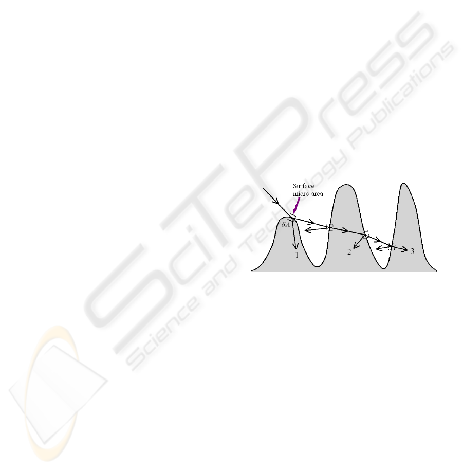
Light transmission processes at a rough surface can
be classified into single and multiple scattering. In
single scattering (ray 1 in Figure 2), a light ray is
scattered one time (this is in fact a refraction at the
local area). In multiple scattering (ray 2 or 3 in
Figure 2), there are multiple times of reflection and
transmission. The total BTDF may be expressed as
total single multiple
ρ
ρρ
=+ , (2)
where
single
ρ
and
multiple
ρ
are the contributions from
single and multiple scattering, respectively.
Figure 2: Light transmission processes of single scattering
(ray 1) and multiple scattering (rays 2 and 3).
Now we use the statistical ray method proposed
by Sun (2007) to calculate light transmission at a
rough surface. The assumptions and conditions of
our considered surface are similar to those used by
Sun (2007) where the focus was on reflection, but
now the focus is on transmission. For convenience,
the assumptions are listed below:
1. Any surface micro-area
A
δ
has size much larger
than wavelength and is sufficiently smooth such
that it can be replaced with its local tangent plane.
2. Any local illumination area
A
Δ
for the definition
of BTDF (Figure 1) contains many surface micro-
areas
A
δ
. As a result, it is valid to use the concept
of probability of micro-areas
A
δ
within
A
Δ .
3. The surface properties remain the same in
A
Δ
.
These properties include the material aspect such
as the optical constants, and the geometric aspect
such as the statistics of the surface profile.
GRAPP 2007 - International Conference on Computer Graphics Theory and Applications
78
4. The surface profile is a height field. That is, for
any line parallel with the z-axis, the line will
intersect with the surface profile exactly one time.
5. A combined probability can be approximated as a
product of the individual probabilities (see below).
6. The correlation between the incident and outgoing
directions are ignored.
As additional conditions, we assume that the surface
is isotropic and has a Gaussian height probability
density and correlation function.
Since the surface is a Gaussian height field, the
probability density function of surface height is
22
1
( ) exp( 2 )
2
p
ζ
ζσ
πσ
=−, (3)
where
ζ
is the surface height, and
σ
is the
standard deviation or RMS.
To describe surface roughness, we need to
consider the surface height correlation. A two-point
correlation function is generally defined as
2
00
() ( )( )Chh
σ
=< + >rrrr, (4)
which involves the average of the product of heights
at points
0
r and
0
+rr on the 0z = plane. Since the
surface is homogeneous (Assumption 3), the
correlation is independent of
0
r
. Also, because the
surface is isotropic, we can write
() ()CCr=r . A
common form of
()Cr is Gaussian, i.e.
22
( ) exp( )Cr r
τ
=− , (5)
where
τ
is the correlation length. Now we define
the surface smoothness as
/s
τ
σ
= . (6)
The smaller is
s
, the rougher the surface; vice versa.
Given surface profile
(, )hxy
ζ
= , the orientation
of a micro-area
A
δ
is described by the partial
derivatives
(, )
x
y
ζζ
′′
(, )
x
hxy
x
ζ
∂
′
=
∂
,
(, )
y
hxy
y
ζ
∂
′
=
∂
. (7)
From Sun (2007), the probability for the orientation
of a micro-area
A
δ
in
x
y
dd
ζζ
′
′
is
222
223
tan
(, ) exp
44cos
nn
xy x y
n
d
pdd
ττθ
ζζ ζ ζ
π
σσθ
⎛⎞
Ω
′′ ′ ′
=−
⎜⎟
⎝⎠
(8)
where
n
dΩ is differential solid angle of (, )
nn
θ
ϕ
n ,
sin
nnnn
ddd
θ
θϕ
Ω=
. (9)
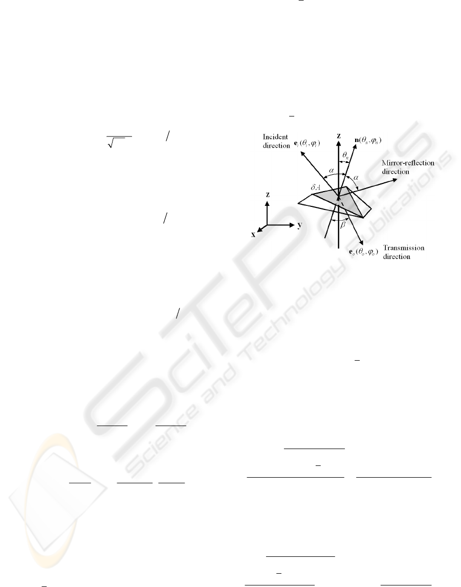
Given a micro-area
A
δ
(Figure 3), the incident
radiance
(, )
iii
L
θ
ϕ
and the transmitted radiance
(, )
oo o
L
θ
ϕ
are related as,
(, )cos
(,) (, )(,, )cos
ooo o
tiiiio i
Ld
FL d
θϕ β
αλ θϕ δ α
Ω
=Ωne e
(10)
where
β
is the transmission angle for the incident
angle
α
,
o
dΩ is the solid angle in the transmission
direction,
i
d
Ω
is the solid angle in the incident
direction, and
(,)
t
F
α
λ
is the Fresnel coefficient of
transmission averaged over polarizations.
(, , )
io
δ
ne e
is a Dirac delta function. That is, when
n ,
i
e , and
o
e are coplanar and
sin sinn
α
β
=
( n is the relative
index of refraction),
(, , ) 1
io
δ
=ne e ; otherwise,
(, , ) 0
io
δ
=
ne e . The radiant flux (, )
oo
δ
θϕ
Φ through a
micro-area
A
δ
is given as
(, ) (, )cos
(,) (, )(, , )cos
oo ooo o
tiiiio i
LAd
FL Ad
δθϕ θϕ βδ
αλ θϕ δ αδ
Φ= Ω
=
Ωne e
(11)
Figure 3: Ray transmission at a micro-area.
Since a local illumination area
A
Δ over which
the BTDF is defined (Figure 1) contains many
micro-areas
A
δ
, the total radiant flux over
A
Δ
contains contributions from all possible micro-areas,
(, ) ( ) (, )
(, )cos ( )(,)(,, )
oo oo
A
iii i t io
A
VA
L
dVAF A
θϕ δ δ θϕ
θ
ϕα δ αλδ δ
Δ
Δ
ΔΦ = Φ
=Ω
∑
∑
ne e
(12)
where
()VA
δ
is a visibility function describing the
probability of a micro-area
A
δ
that is visible in both
directions
(, )
ii i
θ
ϕ
e and (, )
ooo
θ
ϕ
e . The radiance to
the transmission direction
(, )
ooo
θ
ϕ
e
is given as
(, )
(, )
|cos |
(, )cos (,) ( )(,, )
|cos |
oo
ooo
oo
iii it io
A
oo
L
Ad
L
dF VA A
dA
δ
θϕ
θϕ
θ
θ
ϕα αλ δδ δ
θ
ΔΦ
=
ΔΩ
Ω
=
ΩΔ
∑
ne e
(13)
Because
o
θ
is measured from the positive z-axis
(see Figure 1) and its value is within
[/2,]
π
π
, we
take the absolute value of its cosine value in Eq. (13).
Substituting Eq. (13) into Eq. (1), we obtain
single
(over ) (fixed )
(, )
(, )cos
cos ( , ) ( , , )
()
cos | cos |
oo o
iii i i
tio
ioo
L
Ld
FA
VA
dA
ζζ
θϕ
ρ
θϕ θ
α
αλ δ δ
δ
θθ
=
Ω
=
ΩΔ
∑∑
ne e
(14)
Here the summation over the local illumination area
A
Δ
has been decomposed into the summation over
all micro-areas with fixed height
ζ
and over
REALISTIC TRANSMISSION MODEL OF ROUGH SURFACES
79
different heights. Since the visibility function
()VA
δ
at a fixed height remains the same for given incident
and outgoing directions, it has been put outside the
inner summation for a fixed height. Considering that
the projected area of
A
δ
on the 0z = plane is
() cos
n
AA
δ
δθ
⊥
= , (15)
where
n
θ
is the polar angle of the normal (, )
nn
θ
ϕ
n
of
A
δ
(see Figure 3), the portion of the total
projected areas
(fixed )
()(,,)
io
A
ζ
δδ
⊥
∑
ne e in
A
Δ is the
probability of a surface point with height in
differential interval
[, ]d
ζ
ζζ
+
and with orientation
in intervals
[, ]
x
xx
d
ζ
ζζ
′′ ′
+
and [,
y
ζ
′
]
yy
d
ζ
ζ
′′
+
. Thus,
(fixed )
1
()(,,) (,,)
io x y x
A
pddd
A
ζ
δ
δζζζζζζ
⊥
′′ ′ ′
=
Δ
∑
ne e
(16)
From Assumption 5, the combined probability
density function can be decomposed as
(,,) ()(,)
x
yxy
ppp
ζ
ζζ ζ ζζ
′
′′′
=
. (17)
Applying Eqs. (16,17) into Eq. (14), we obtain
222
single
4
cos ( , ) exp( tan 4)
4 cos | cos | cos
()(, , )
tn
io n
n
io
o
sF s
d
dp V
d
ααλ θ
ρ
πθ θ θ
ζζ ζ
−
=
Ω
⋅
Ω
∫
ee
(18)
This equation may be further expressed as
222
single
4
cos ( , ) exp( tan 4)
4 cos | cos | cos
(, ) (,, )
tn
io n
io
sF s
V
ζ
ααλ θ
ρ
πθ θ θ
χαβ ζ
−
=
⋅ ee
(19)
where the function
(, )
χ
αβ
describes
no
ddΩΩ (see
Appendix), and
(,,) ()(,,)
io io
VdpV
ζ
ζζζζ
=
∫
ee ee (20)
is the averaged bistatic visibility function. A bistatic
visibility function simultaneously involves the
incident direction
i
e and the outgoing direction
o
e .
For light transmission, since
i
e points into the
original medium and
o
e into the new medium, the
correlation between the two directions can be
ignored, as stated in Assumption 6. Therefore,
(, , ) (, )(, )
io i o
VVV
ζ
ζθ ζθ
≈ee
, (21)
where
(,)V
ζ
θ
is an individual visibility function that
describes the probability of being visible for a ray
starting at height
ζ
and with angle
θ
(Figure 4),
and accordingly,
(, , ) (, )(, )
()(, )(, )
io i o
io
VVV
dp V V
ζζ
ζζθζθ
ζ
ζζθζθ
≈
=
∫
ee
(22)
We further approximate Eq. (22) as
(, , ) (0, )(0, )
io i o
VVV
ζ
ζ
θθ
≈ee
. (23)
where
(0, )
i
V
θ
and (0, )
o
V
θ
are the individual
visibility functions for the incident and outgoing
directions when the ray starts from
0
ζ
= . From the
previous study (Sun, 2007),
()
22
0
tan
(0, ) exp exp 4tan
k
Vs
s
θ
θ
θ
⎡
⎤
≈− −
⎢
⎥
⎣
⎦
,(24)
where
0
0.7k = . Thus, we finally obtain
222
single
4
cos ( , )exp( tan 4)
4 cos | cos | cos
(,)(0, )(0, )
tn
io n
io
sF s
VV
ααλ θ
ρ
πθ θ θ
χαβ θ θ
−
=
⋅
(25)
where
(, )
χ
αβ
is given in the Appendix.
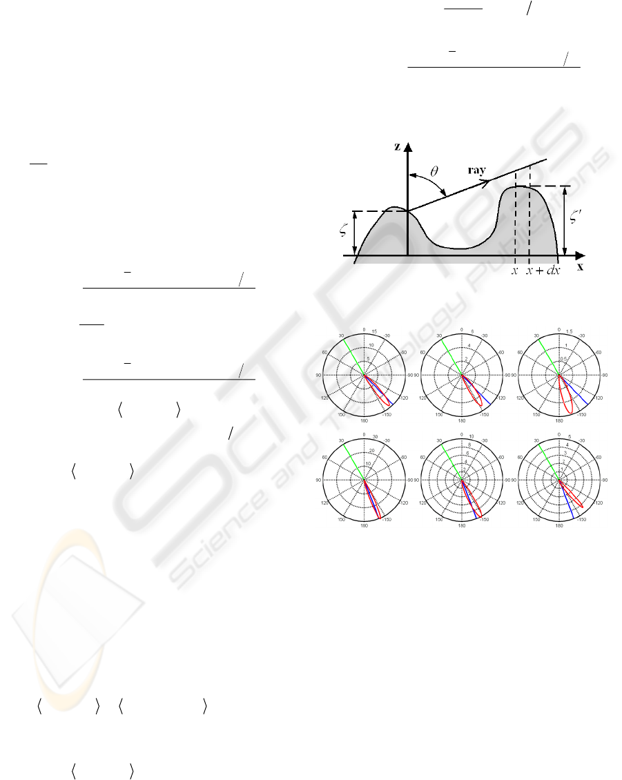
Figure 4: A ray starts at height
ζ
and with polar angle
θ
.
Figure 5: BTDF for different n and
s
. Parameters are
30
i
θ
=
° , 1/1.4n
=
for the first row, and 1.4n = for the
second row. From the left to right, the values of
s
are 6, 3,
and 1, respectively.
Figure 5 shows
single
ρ
for different values of
relative index of refraction (IOR)
n and smoothness
s
. The solid straight lines (in green) in the upper
hemisphere indicate the incident direction, and the
solid straight lines (in blue) in the lower hemisphere
indicate the transmission direction.
single
ρ
has a sharp
lobe and shows the off-specular effect. When
1n
<
(the first row), as the outgoing direction changes
from
90
θ
=
−° to 180
θ
=
° ,
single
ρ
increases gradually
and reaches a maximum, then decreases rapidly.
GRAPP 2007 - International Conference on Computer Graphics Theory and Applications
80
Also, the direction that
single
ρ
has the maximum
shifts toward
180
θ
=° with the decrease of
s
. In
contrast, for
1n > (the second row), when the
outgoing direction changes from
90
θ
=− ° to
180
θ
=°,
single
ρ
increases rapidly and reaches the
maximum, then decreases gradually. Moreover, the
direction for the maximum
single
ρ
shifts toward
90
θ
=− ° with the decrease of
s
.
The plots in Figure 5 can be explained as below.
First, when the surface is smooth, most micro-areas
distribute around
0
n
θ
=° and they contribute to
single
ρ
with
i
α
θ
→
. Second, Fresnel’s transmission
coefficient has the maximum for incident angle
0
α
=°, and decreases with the increase of
α
.
Therefore, those micro-areas with orientation around
the incident direction have large Fresnel’s
transmission coefficients. These two factors compete
with each other. And also, for
1n < , the refraction
angle
β
is larger than the incident angle
α
, and
vice versa. These result in the plot shapes in Figure
5. With the decrease of
s
, the maximum distribution
of orientations of micro-areas tends to shift from
0
n
θ
=° toward 90
n
θ
=°, which results in a shift of
the direction for the maximum
single
ρ
.
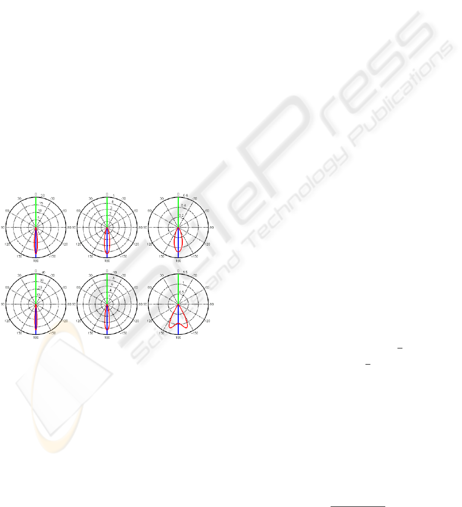
Figure 6: BTDF for different n and
s
. Here 0
i
θ
=
° , and
other parameters and notations are the same as Figure 5.
For the normal incidence,
single
ρ
for different
values of
n and
s
is shown in Figure 6. For 1n
<
,
the sharp lobe becomes wider with the decrease of
s
, as same as Figure 5. However, for the case 1n >
in both Figures 5 and 6, although the sharp lobes for
3s = are all wider than those for 6s = , the sharp
lobes for
1s = have different shapes. Consider the
rotational geometry,
single
ρ
for 1s = in Figure 6 is
actually a lobe with an indented peak. We can
understand this by the micro-area model. For rough
surfaces (
1s = ), most micro-areas distribute with
orientations
0
n
θ
° , and therefore the transmitted
light by single scattering tends to travel along the
direction with
90 180
o
θ
°° . This results in the
indentation of the lobe in Figure 6. However, the
probability of ray blocking is higher for the rays
propagating along this direction. This results in the
sharper shape for
1s
=
in Figure 5.
4 NUMERICAL SIMULATION
In our Monte Carlo simulation, given a Gaussian
rough surface with its mean equal to zero and
standard deviation
σ
, totally
N
light rays are shot
from the incident direction
i
e , each ray carrying a
weight
l
W
( 1, 2,...,lN
=
) that represents its radiance
flux intensity. Once a shot ray hits the surface
profile, it typically splits into a reflected and a
transmitted ray. When the total internal reflection
occurs, only a reflected ray is generated.
The surface height at which a shot ray intercepts
with the profile is determined by the probability
density function of surface height and a generated
random number (all the generated random numbers
in this paper are uniformly distributed between 0 and
1). The normal direction of this intersection point is
obtained by the orientation probability density
function with two generated random numbers.
We set the incident flux density to 1. Then the
weight of the lth shot ray is given as
1
( , )cos / cos
li n
WV
ζ
θαθ
=
, (26)
where
1
ζ
is the surface height that the shot ray first
intercepts with,
α
is the incident angle in the local
area, and
cos
n
θ
is involved because Eq. (16) just
describes the probability distribution of
A
δ
⊥
at a
fixed height.
When a ray with weight
W hits the surface
profile, it splits into a reflected and transmitted ray,
and the weight of the reflected ray is
(,)
r
FW
αλ
and
that of the transmitted ray is
(,)
t
FW
αλ
. Therefore,
after each ray splitting, the generated rays will
decrease in intensities. Once the weight of a newly
generated ray is lower than the threshold, the
tracking process terminates. Otherwise, it will be
tracked continuously; whether it is blocked or not
depends on its propagation direction, visibility
function, and a generated random number.
The radiance to the transmission direction
(, )
ooo
θ
ϕ
e is obtained as
|cos |
o
l
l
o
oo
W
L
N
θ
∈ΔΩ
=
ΔΩ
∑
, (27)
REALISTIC TRANSMISSION MODEL OF ROUGH SURFACES
81
where
o
ΔΩ is the solid angle along (, )
ooo
θ
ϕ
e , and
o
l
l
W
∈ΔΩ
∑
calculates the sum of the weights of those
rays transmitted into
o
ΔΩ . Consider that the incident
irradiance is
cos
i
θ
(since incident flux density is set
to 1), the BTDF can be calculated by
|cos |cos
o
l
ooi
W
N
ρ
θ
θ
ΔΩ
=
ΔΩ
∑
. (28)
In discussion below we may replace
ρ
with
|cos |
o
ρ
θ
based on two considerations. First, the
previous simulations by Nieto-Vesperinas et al.
(1990) calculated the transmitted light intensity,
which is proportional to
|cos |
o
ρ
θ
. For convenience
of comparing the results, we need to use
|cos |
o
ρ
θ
instead of
ρ
. Second, Eq. (28) contains
1/ | cos |
o
θ
and
o
l
l
W
∈ΔΩ
∑
. When
o
θ
π
→
,
|cos | 0
o
θ
→
. However,
we cannot take
0
o
ΔΩ →
for the calculation of Eq.
(28). Therefore,
ρ
might diverge at 90
o
θ
→°.
Figure 7: Comparison between our analytical model and
simulations. The curves with x marks are from the
analytical model, the dot curves from the simulations of
Nieto-Vesperinas et al. (1990), and the solid curves from
our simulations. Here,
1.411n = , 2.522s = , (a) 0
i
θ
=
° , (b)
20
i
θ
=°, (c) 40
i
θ
=°, and (d) 60
i
θ
=°.
Figure 7 compares our analytical model and
simulations. Nieto-Vesperinas et al. (1990)
considered perpendicular and parallel polarizations
separately. For comparison, we calculate the average
of the two polarizations. In our analytical model and
simulation, light intensity can be calculated by
|cos |
o
A
ρθ
Δ . Since we do not know the value of
A
Δ used for the simulation of Nieto-Vesperinas et
al., we find it by matching our analytical model with
their results for
0
i
θ
=
° . In Figure 7, the comparison
shows a very good match.
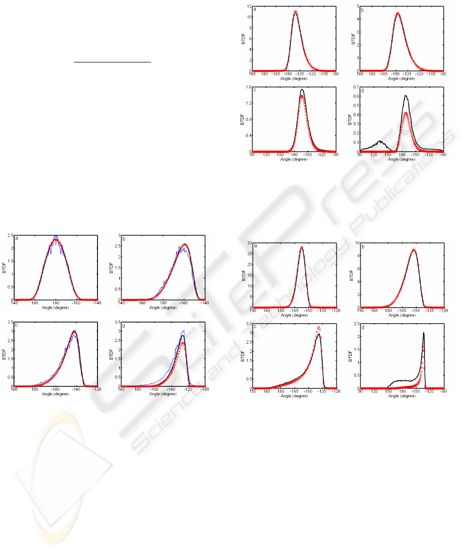
Figure 8: Comparison between simulation and analytical
model. The solid curves are from our simulation, and the
curves with x marks from analytical model. Here,
30
i
θ
=
° ,
1/1.4n =
, (a)
6s
=
, (b)
3s =
, (c)
1s =
, and (d)
0.5s
=
.
Figure 9: Comparison between simulation and analytical
model. The solid curves are from our simulation, and the
curves with x marks from analytical model. Here,
30
i
θ
=
° ,
1.4n =
, (a)
6s
=
, (b)
3s
=
, (c)
1s =
, and (d)
0.5s =
.
Figures 8 and 9 compare our simulation and the
analytical model for different values of
n and
s
.
For smooth and moderately smooth surfaces (
s
is 3
or 6), the analytical model agrees well with the
simulation. With small
s
, the difference between
the analytical model and simulation increases. This
is because our analytical model only considers single
scattering. For smooth surfaces, light transmission is
dominated by single scattering. Overall, the model
has a good match with the simulation. For rough
surfaces (
s
is small), multiple scattering plays an
important role and should be considered.
GRAPP 2007 - International Conference on Computer Graphics Theory and Applications
82

5 CONCLUSIONS
This paper presents a realistic transmission model of
rough surfaces. The model is derived based on the
statistical ray method. We have obtained an
analytical expression for single scattering. The
model has been compared to our Monte Carlo
simulations as well as to the simulations by others,
and good agreements have been achieved.
In future work, the model can be applied to
render realistic transmission effects. The model
could be taken into consideration to study object
translucency. On simulation to verify the analytical
model, we may generate 2D surfaces for given
σ
and
τ
, and compute the average of transmission
through the surfaces. The current model has not
considered multiple scattering, and both the model
and simulation have not considered polarization
effects. We will consider them in our further work.
REFERENCES
Ashikhmin, M., Premoze, S., Shirley, P., 2000. A
microfacet-based BRDF generator. In
Proc. of ACM
SIGGRAPH
, pp. 65-74.
Beckmann, P., Spizzichino, A., 1963.
The Scattering of
Electromagnetic Waves from Rough Surfaces
,
Macmillan, New York.
Blinn, J. F., 1977. Models of light reflection for computer
synthesized pictures. In
Proc. Siggraph, pp. 192-198.
Cook, R. L., Torrance, K. E., 1982. A reflection model for
Computer Graphics.
ACM Transactions on Graphics,
vol. 1, no. 1, pp. 7-24.
Dorsey, J., Edelman A., Jensen H. W., Legakis J., and
Pedersen H. K., 1999. Modeling and rendering of
weathered stone. In
Proc. Siggraph ‘99, pp. 225-234.
Fung, A. K., Chen, M. F., 1985. Numerical simulation of
scattering from simple and composite random
surfaces.
J. Opt. Soc. Am. A, vol. 2, no. 12, pp. 2274-
2284.
Glassner, A. S., 1995.
Principles of Digital Image
Synthesis
, Morgan Kaufmann Publishers, San
Francisco, CA.
Hanrahan, P., and Krueger W., 1993. Reflection from
layered surface due to subsurface scattering. In
Proc.
Siggraph ‘93
, pp. 165-174.
He, X. D., 1993. Physically-based models for the
reflection, transmission and subsurface scattering of
light by smooth and rough surfaces, with applications
to realistic image synthesis. Ph.D thesis, Cornell
University, Ithaca, New York.
He, X. D., Torrance, K. E., Sillion, F. X., Greenberg, D.
P., 1991. A comprehensive physical model for light
reflection. In
Proc. Siggraph, pp. 175-186.
Jensen, H. W., and Christensen P. H., 1998. Efficient
Simulation of Light Transport in Scenes with
Participating Media Using Photon Maps.
Computer
Graphics Proceedings (Proc. SIGGRAPH ’98
), pp.
311-320.
Jensen H. W., Marschner S. R., Levoy M., and Hanrahan
P., 2001. A practical model for subsurface light
transport. In
Proc. Siggraph ‘01, pp. 511-518.
Jensen H. W., and Buhler J., 2002. A rapid hierarchical
rendering technique for translucent materials.
ACM
Trans. Graph.
21, vol. 3, pp. 576-581.
Koenderink J., and Doorn A. van., 2001. Shading in the
case of translucent objects. In
Proc. SPIE, vol. 4299,
pp. 312-320.
Kubelka, P., and Munk, F., 1931. Ein Beitrag Zur Optik
Der Farbanstriche, Zeitschrift fr Technishen Physik, p.
593.
Lafortune, E. P. F., Foo, Sing-Choong, Torrance, K. E.,
Greenberg, D. P., 1997. Non-linear approximation of
reflectance functions. In
Proc. Siggraph, pp. 117-126.
Mertens, T., Kautz, J., Bekaert, P., Reeth, F. V., and
Seidel, H. –P., 2005. Efficient rendering of local
surface scattering. In
Computer Graphics Forum, vol.
24, pp. 41-49.
Nieto-Vesperinas, M., Sanchez-Gil, J. A., Sant, A. J.,
Dainty, J. C., 1990. Light transmission from a
randomly rough dielectric diffuser: theoretical and
experimental results.
Opt. Lett., vol. 18, no. 22, pp.
1261-1263.
Pharr, M., and Hanrahan, P., 2000. Monte carlo evaluation
of non-linear scattering equations for subsurface
reflection. In
Proc. Siggraph ‘00, pp. 75-84.
Phong, B., 1975. Illumination for computer generated
images.
Comm. of ACM, vol. 18, no. 6, pp. 311-317.
Stam, J., 2001. An illumination model for a skin layer
bounded by rough surfaces. In
Proceedings the 21th
Eurographics Workshop on Rendering Techniques
, pp.
39-52.
Sun, Y., 2007. Analytical framework for calculating
BRDFs of randomly rough surfaces.
J. Opt. Soc. Am.
A
, (to appear in March 2007). Currently available
online at http://josaa.osa.org/upcoming.cfm.
Torrance, K. Sparrow, E. M., 1967. Theory for off-
specular reflection from roughened surfaces.
J. Opt.
Soc. Am.
, vol. 57, no. 9, pp. 1105-1114.
Ward, G. J., 1992. Measuring and modeling anisotropic
reflection. In
Proc. SIGGRAPH, pp. 265-272.
Wang, R., Tran, J., and Luebke, D., 2005. All-Frequency
Interactive Relighting of Translucent Objects with
Single and Multiple Scattering, in ACM Trans.
Graphics (Proc. SIGGRAPH ’05), pp. 1202-1207.
APPENDIX
Here we derive the relationship between the
differential solid angles
o
d
Ω
and
n
dΩ . Given an
unit sphere (Figure 10), the area
A
BCD corresponds
to
n
d
Ω
and the area
A
BCD
′
′′′
to
o
dΩ . The points
A
,
B
,
A
′
, and
B
′
are coplanar, and similarly the
points
C , D , C
′
, and D
′
. The planes
A
BA B
′
′
and
DCD C
′
′
intersects at the line POQ , and the angle
REALISTIC TRANSMISSION MODEL OF ROUGH SURFACES
83

between them is
d
γ
. Therefore, the length of the
curve segment
A
D is
|||| sin
A
DAEd d
γ
αγ
=⋅=⋅
. (A1)
Since
||
A
Bd
α
= , so we obtain
||||sindADAB dd
α
γα
Ω= ⋅ = ⋅
. (A2)
(a)
(b)
Figure 10: Relationship between
n
dΩ and
o
dΩ ( 1n > ).
The Snell’s law gives the following relations:
sin sinn
α
β
=⋅ (A3)
and
sin sin( ) sin sin( )dn n d
α
αα β ββ
′′
=+=⋅=⋅+
, (A4)
where
n is the relative index of refraction ( 1n > )
and
d
β
is defined as
d
β
ββ
′
=−
. (A5)
From Eq. (A4), we can obtain
sincos()cossin()
[sin cos( ) cos sin( )]
dd
nd d
αααα
β
βββ
⋅+⋅
=⋅ ⋅ + ⋅
(A6)
We make the following approximations:
cos( ) 1, sin( ) ,
cos( ) 1, sin( ) .
ddd
ddd
α
αα
β
ββ
≈≈
≈≈
(A7)
Substituting Eqs. (A3) and (A7) into Eq. (A6), we
obtain
cos
cos
dd
n
α
β
α
β
=
⋅
. (A8)
From Figure 10(b), we obtain
A
OB d
β
βα
′
′′
=
−∠ + . (A9)
Therefore, we obtain
cos
1
cos
A
OB d
n
α
α
β
⎛⎞
′′
∠=−
⎜⎟
⋅
⎝⎠
. (A10)
The length of the curve segment
A
B
′′
is
cos
|| 1
cos
A
BAOB d
n
α
α
β
⎛⎞
′′ ′ ′
=∠ = −
⎜⎟
⋅
⎝⎠
. (A11)
The length of the curve segment
A
D
′′
is
||||
sin( ) sin( )
AD AE d
A
OQ d d
γ
γ
αβγ
′
′′′
=⋅
′
=∠ = −
(A12)
Therefore, we obtain
0
||||
cos
1sin()
cos
dABAD
dd
n
α
α
βγα
β
′′ ′′
Ω= ⋅
⎛⎞
=− −
⎜⎟
⎝⎠
(A13)
Finally, we obtain
1
sin cos
(, ) 1
sin( ) cos
n
o
d
dn
αα
χαβ
αβ β
−
⎛⎞
Ω
≡= −
⎜⎟
Ω−⋅
⎝⎠
(A14)
Although Eq. (A14) is derived for
1n > , it is easy to
prove that this expression also holds for
1n < .
GRAPP 2007 - International Conference on Computer Graphics Theory and Applications
84
