
DETECTING FEATURES FROM SLICED POINT CLOUDS
Ioannis Kyriazis, Ioannis Fudos and Leonidas Palios
Department of Computer Science, University of Ioannina, Ioannina, Greece
Keywords:
Reverse Engineering, Feature-Based CAD Models, Cross-Sections, Point Cloud, Convex Hull, Voronoi Dia-
gram.
Abstract:
We present a new method for extracting the feature primitives of a 3D object directly from the point cloud of
its surface scan. The objective is to identify a subset of points that provides the same information about the
structure and the topology of the object geometry as the point cloud itself. The entire process is carried out
with the least human intervention possible. The only information we receive as input is the point cloud of the
3D scan of the object.
First, the point cloud is sliced in cross sections. Each cross section consists of a 2D point cloud.
A collection of curve patches is derived for each slice, describing the cross section, and providing a feature-
based CAD model appropriate for further editing. For the extraction of the feature points and the interpolating
curve patches we use properties of the convex hull and the voronoi diagram of the point cloud.
1 INTRODUCTION
Many applications in manufacturing, medicine, geog-
raphy, design, etc. require the scanning of 3D ob-
jects to incorporate them into a computer-based or
computer-aided processing system, with a technique
known as Reverse Engineering. Advanced measur-
ing techniques have been developed to produce a large
amount of points lying on the object surface, i.e. the
point cloud of the object.
We present a method for dividing the point cloud
into several slices, which are processed separately and
provide local information about the object. This infor-
mation is used to extract local features of the object.
Such features may include holes or extrusions on the
object, symmetrical or similar parts, and also scaled,
flipped and generally transformed versions of already
known features.
Several methods have been developed that extract
features from a point cloud. (Jeong et al., 2002) use
an automated procedure to fit a hand-designed generic
control mesh to a point cloud of a human head scan.
A hierarchical structure of displaced subdivision sur-
faces is constructed, which approximates the input
geometry with increasing precision, up to the sam-
pling resolution of the input data. (Au and Yuenb,
1999) use a method that fits a generic feature model
of a human torso to a point cloud of a human torso
scan. The features are recognized within the point
cloud by comparison with the generic feature model.
This is achieved by optimizing the distance between
the point cloud and the feature surface, subject to con-
tinuity requirements. (Amenta et al., 1998) proposed
the crust algorithm, which combines the point cloud
with the vertices of the Voronoi diagram, and com-
putes the Delaunay tetrahedralization of the combined
point set. The triangles where all vertices are sample
points (not voronoi vertices) are considered to form
the object surface. (Attene and Spagnuolo, 2000) use
some properties of geometric graphs. The EMST is
used as a constraint during the sculpturing of the De-
launay tetrahedronization of the data set, and in addi-
tion another constraint is used, the so-called Extended
Gabriel Hypergraph (EGH). These methods are fast
and general but do not provide models appropriate for
CAD use.
Our method uses a subset of the point cloud each
time, which is then used to extract a feature locally.
188
Kyriazis I., Fudos I. and Palios L. (2007).
DETECTING FEATURES FROM SLICED POINT CLOUDS.
In Proceedings of the Second International Conference on Computer Graphics Theory and Applications - GM/R, pages 188-192
DOI: 10.5220/0002082701880192
Copyright
c
SciTePress
This is accomplished by dividing the point cloud into
several slices. These slices contain the same informa-
tion as the initial point cloud - the (x, y, z) coordinates
of the points - with the additional information that the
points of a slice are located near a planar surface that
intersects the object at a specific direction. The points
of each slice can be considered to be co-planar, and
so we can process each slice as a 2D set of points, in-
stead of a 3D object. This provides for more efficient
and accurate local feature extraction.
The local per slice feature representation is then
combined with information provided from several ad-
jacent slices, to reconstruct the global structure and
morphology of the object.
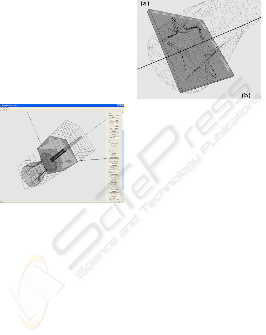
Figure 1: A point cloud can be sliced in any desired direc-
tion. Slice thickness is determined adaptively.
2 SLICING THE POINT CLOUD
A major issue of the point cloud segmentation is
the slicing direction. The direction along which we
choose to divide the object into slices may influence
the process of feature extraction and the resulting
model. To this end we can either align interactively
the object to the desired direction, or seek automati-
cally a transformation of the object that minimizes a
target function, e.g. PCA.
Another key issue is to determine the proper thick-
ness for a slice. The points of a very thick slice may
not provide useful information, as we might get many
features tangled together. To avoid this we can split
it into two new slices with reduced thickness. On the
other hand, the points of a very thin slice may be in-
adequate to describe a feature, or the points of two ad-
jacent slices may carry almost the same information,
so we can merge the two slices into one slice with in-
creased thickness. We could also determine the ideal
Figure 2: (a) A slice of the cloud is highlighted. (b) The
points of the slice are projected on a plane parallel to the
slice.
slice thickness adaptively, as described in (Wu et al.,
2004). The distance between two slices can also be
a parameter, but as we do not want to omit any in-
formation from points located between two slices, we
set each slice to start exactly where the previous slice
ends (and there is no empty space between adjacent
slices).
Once we have divided the point cloud into slices,
the points that belong to each slice are projected on
a plane that is vertical to the slicing direction, so we
can use 2D techniques for processing the points of the
slice. Figure 1 illustrates an example of a sliced point
cloud of a Screwdriver, and Figure 2 shows the points
of a slice, and the projected point cloud slice. Figure 1
also shows the interface of the prototype that we have
developed to test our method.
The next objective is to reduce the number of
points, since we can extract the desired information
from only a small point subset. These feature points
are identified with the method described in the next
section.
3 IDENTIFYING FEATURE
POINTS ON A SLICE
The initial point cloud consists of a very large number
of points, depending on the size and shape of the pro-
totype object, and also on the accuracy that was used
to scan the object. The large number of points makes
it difficult to process this raw information. Thus, we
need to reduce the number of points in the cloud while
retaining all the information provided by these points.
If the points of a slice formed a 2D shape that was
convex then we simply compute the convex hull of
DETECTING FEATURES FROM SLICED POINT CLOUDS
189
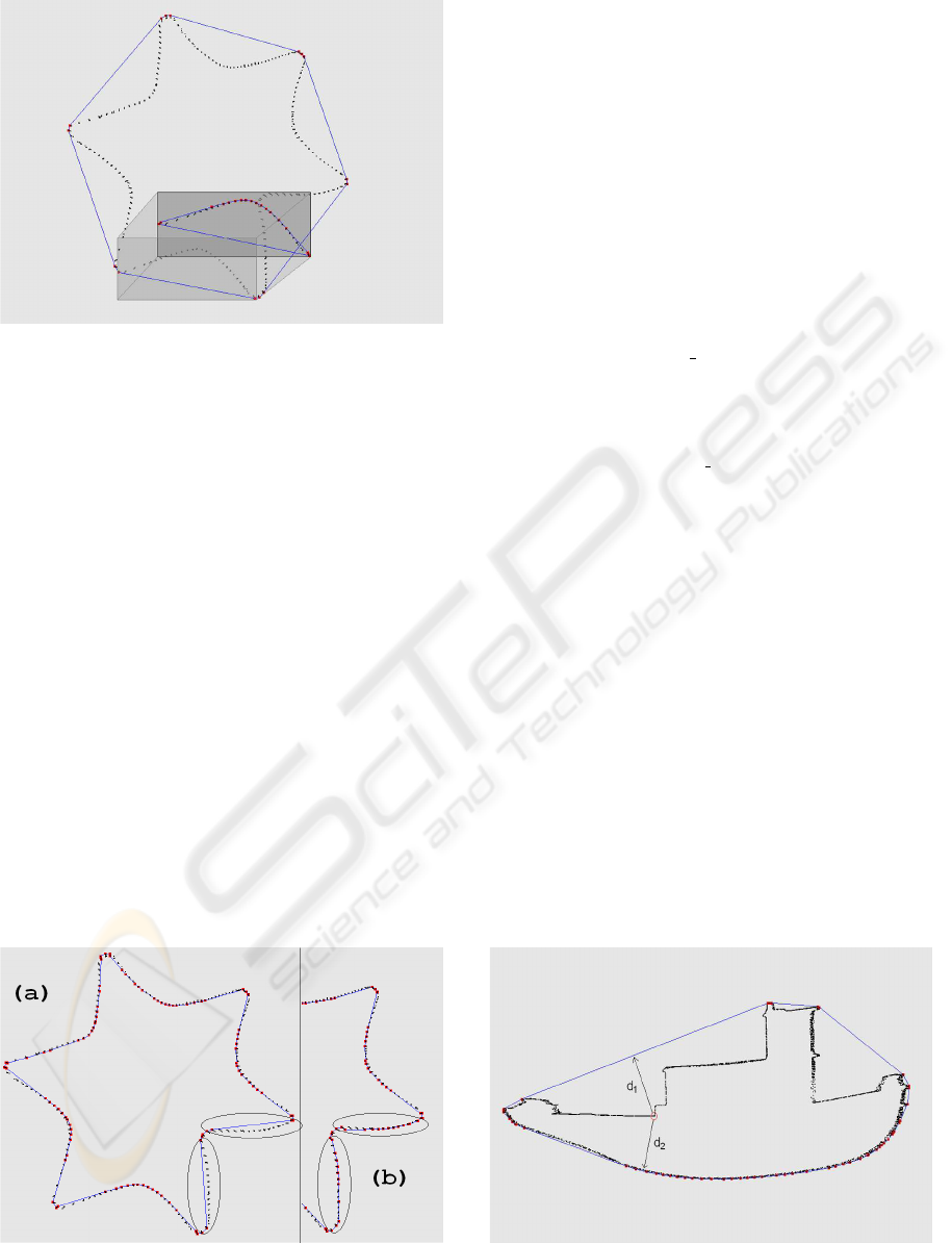
Figure 3: The points in the highlighted region are isolated
and the convex hull of these points is computed to identify
the next set of feature points for the curve.
the points to describe the shape with a polyline con-
sisting usually of much fewer vertices than the points
in the slice. But in general the shape of the points in a
slice is not convex, and thus to interpolate a curve to
these points we need more than just the convex hull of
the points. We always start by computing the convex
hull of the points, to identify some of the points that
will form the curve that best fits our point slice. Now
there are points that are located near the convex hull
(up to a threshold), while other points are still located
far from the convex hull. We partition the points in
regions, one for each line segment of the convex hull.
Some regions may consist exclusively of points near
the convex hull, and other regions consist of points
located far from it. We treat further these remote re-
gions by computing the convex hull of their points,
and then we repeat the same process as for the initial
object (this is illustrated in figure 3). By combining
the initial convex hull with the convex hull of each
region, we get a curve that interpolates the points of
Figure 4: (a) First step of the Convex Hull Method. There
are still some regions where the curve doesn’t fit the points
accurately. (b) Second Step of the Convex Hull Method.
The curve now describes the slice points more accurately.
the slice adequately in most regions. We repeat com-
puting the convex hull for the rest of the regions until
all regions consist of points that are located near the
curve (for a termination criterion see (Said, 2002)).
An example is illustrated in Figure 4.
The method, as applied to a specific slice, is sum-
marized as follows:
Input: a set
P
of points, Slice
i
Output: an ordered set
F
i
of feature points
step 1:
(P
(3D)
i
, L) = slice(i, P)
step 2:
P
i
= project(P
(3D)
i
, S)
step 3:
F
i
= qconvex(P
i
)
step 4: for each region
P
ij
of
F
i
if
avg dist(P
ij
, F
ij
) > e
F
ij
= qconvex(P
ij
) − F
ij
end if
end for
F
i
= F
i
∪ F
ij
if
changes made = true
repeat step 4
end if
step 5: return
F
i
where L is a plane parallel to the slice where we
project the 3D slice. The method described above
works fast and accurately in most cases, but there are
cases in which the curve interpolating the points of
the slice differs significantly from the object we try to
describe. There are two important issues concerning
the points of a slice that might affect the effectiveness
of the interpolating curve. One is the case when one
or more points are assigned to the wrong region of
the curve. One would expect that each point belongs
to the region of the curve which is closest to the point.
But there may be cases in which a point is closest to
one region, but belongs to another region, for exam-
ple the one that is located on the opposite side of the
closed curve (e.g. see Figure 5). To avoid having such
Figure 5: The points in the highlighted area are located
closer to a region other than the one they should be assigned
to (d
2
< d
1
). We use the information of their neighboring
points to assign them to the correct region.
GRAPP 2007 - International Conference on Computer Graphics Theory and Applications
190
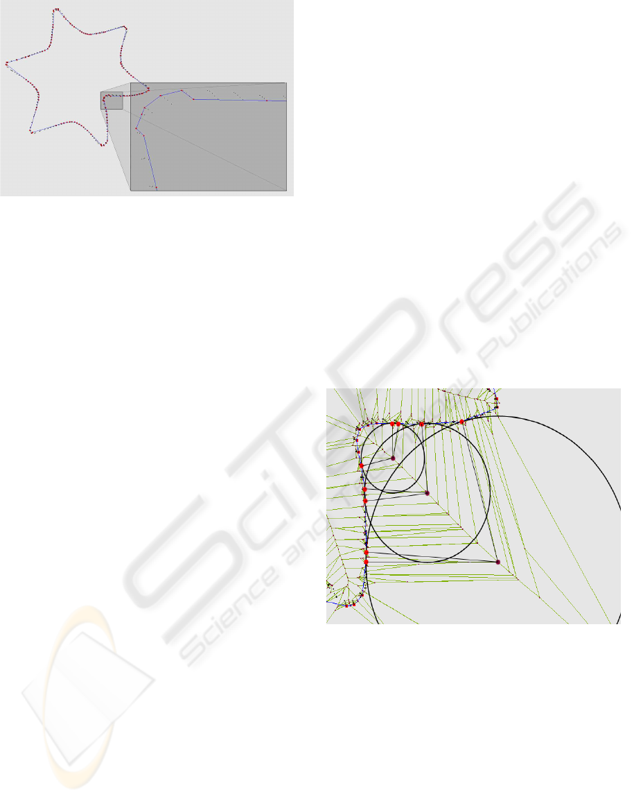
Figure 6: The convex hull method identifies internal and
external slice points alternatively as feature points. If this
affects the curve significantly, we may have to overcome
the switching effect.
false assignments, we keep track of the previous point
assignments, and if one point is found to be closer to
one region, while its neighbors are closer to another,
we ignore the distance to the closest region and as-
sign the point to the region we assigned the neighbor-
ing points. When the distance is close to zero we can
change region.
Another issue is that the point slice is usually ar-
ranged on a wider area rather than a mere curve. Con-
sidering that the points of the 3D cloud lie on the sur-
face of the object, we would expect the points of a 2D
slice to lie on a curve with no thickness. But since we
allow for slices of certain adaptable thickness, pro-
jecting the points on a plane produces point regions
that form a thickened curve. If the dispersion of the
points is insignificant, the resulting curve would be
suitable. If not, computing the convex hull on each re-
gion would result in selecting external points on some
parts of the slice, and internal points on other parts
(see Figure 6). We call this the internal-external point
switching effect. To overcome this effect we use an
alternative approach, which is described in the next
section.
4 ELIMINATING THE
INTERNAL-EXTERNAL POINT
SWITCHING EFFECT
In cases where the points of a slice cover an area sig-
nificantly wider than the curve we try to extract, we
have to extract those points that describe the object
without information loss. Since we started identify-
ing feature points using the convex hull, our concern
is to identify external points only. To achieve this,
we use a property of the voronoi diagram, called the
largest empty circle. If we compute the voronoi di-
agram for the slice points, each voronoi vertex is a
center for a largest empty circle that is touching three
or more slice points. We can use this property on a re-
gion that consists of points which are located far from
the curve, to identify external points of the region.
First, we choose the farthest voronoi vertex lo-
cated on the opposite side of the curve than the region
points, and locate the three (or more) points that are
on the largest empty circle for this vertex. Since we
chose the farthest voronoi vertex, two of these points
are expected to be the extreme feature points of this
region, which are already known from the previous
step. So we expect one or more remaining points to be
identified as new feature points. This is equivalent to
choosing the third point of the unique Delaunay trian-
gle that the two already known feature points partici-
pate in, considering that there aren’t more than three
co-circular points for this voronoi vertex (if there are
more, the triangle is not unique, but still we can
choose any of the points, or all of them). We iden-
tify these new points as feature points and update the
curve accordingly. We repeat the process, until all
points are located near the curve.
Figure 7: The largest empty circle for the farthest voronoi
vertex is used in each step to identify additional feature
points and update the curve.
By choosing the farthest voronoi vertex every
time, the feature points are expected to be relatively
close to each other, as the curve closes in to the region
points slowly. We can ignore some voronoi vertices
that are too far from the region, and choose a voronoi
vertex that is the farthest within a bounded area. For
example, we can choose that voronoi vertex that is far-
ther from the region, but not farther than e.g. the max-
imum distance of the region points from the curve.
This condition is indicative for the speed of the curve
convergence. If we do not restrict the voronoi vertices
it will take many steps to fully update the curve on this
DETECTING FEATURES FROM SLICED POINT CLOUDS
191

region. The curve will consist of more feature points,
and it will describe the region points more accurately.
On the other hand, if we restrict the voronoi vertices
within a radius, it will take fewer steps to update the
curve, the feature points will be fewer, but the curve
would describe the region points less accurately. We
use this parameter to adapt the curve fitting accord-
ing to user specifications requirement or quality of
approximation guaranties. Figure 7 illustrates the re-
sulting curve in case we choose the farthest voronoi
vertex within a restricted area each time. If we had
chosen the farthest voronoi vertex in each step, the
resulting curve would consist of more feature points.
The curve would describe the slice points more accu-
rately, but more iterations would be required to fully
update the curve.
The method, as applied to a specific slice, is sum-
marized as follows (following the notation of Section
3):
Input: a set
P
of points, Slice
i
Output: an ordered set
F
i
of feature points
step 1:
(P
(3D)
i
, L) = slice(i, P)
step 2:
P
i
= project(P
(3D)
i
, L)
step 3:
F
i
= qconvex(P
i
)
step 4: for each region
P
ij
of
F
i
if
avg dist(P
ij
, F
ij
) > e
V
i
= qvoronoi(P
ij
)
V
max
= farthest
vertex(V
i
, P
ij
)
F
ij
= largest circle(V
max
, P
ij
)
end if
end for
F
i
= F
i
∪ F
ij
if
changes made = true
repeat step 4
end if
step 5: return
F
i
5 PERFORMANCE
Both the convex hull and the voronoi diagram require
O(nlogn) operations. Apart from computing the con-
vex hull and the voronoi diagram for each region, the
rest of operations require O(n), where n is the number
of points in the cloud. These operations include: (a)
loading the cloud into memory, (b) slicing the cloud,
and (c) projecting the slice points on the slice. Other
operations that require O(n) are (d) selecting the ap-
propriate voronoi vertex for each region, and (e) to
identify the feature points for that region.
To compute the convex hull and the voronoi di-
agram for each region, it would take O(n
j
logn
j
),
where n
j
is the number of points in region j. This
means that we need O(
∑
r
j=1
n
j
logn
j
) operations for
slice i, where r is the number of regions, and
O(
∑
s
i=1
∑
r
j=1
n
ij
logn
ij
) for all slices, where s is the
number of slices. This is also accomplished in
O(nlogn), since
∑
s
i=1
∑
r
j=1
n
ij
= n.
One issue is the number of iterations required to
fully fit the curve to the slice points. It depends on
the shape of the points, and in the worst case it may
require up to O(logn
i
) steps the n
i
points of slice i,
i.e. O(logn) for all slices. In practice, it usually takes
only a few steps. In the example of Figure 4, the re-
sulting curve is satisfactory after the second step.
In conclusion, to derive descriptive curves for all
slices of the point cloud takes O(nlog
2
n) time.
6 CONCLUSIONS
We have developed a method for representing cross
sections (slices) of a point cloud, which will be used
to identify the basic features of the object this point
cloud represents. The information extraction process
consists of several steps, which involve the segmenta-
tion of the 3D point cloud in 2D cross sections, and
the extraction of a descriptive curve for the corre-
sponding point slice. The extraction of the curve is
performed either by computing the convex hull of the
desired regions of the slice points, or by computing
the convex hull and the voronoi diagram of the slice
points, and use the largest empty circle for voronoi
vertices of insufficiently described regions to identify
exterior feature points.
REFERENCES
Amenta, N., Bern, M., and Kamvysselis, M. (1998).
A new Voronoi-based surface reconstruction algo-
rithm. Computer Graphics, 32(Annual Conference
Series):415–421.
Attene, M. and Spagnuolo, M. (2000). Automatic surface
reconstruction from point sets in space. Computer
Graphics Forum, 19(3):457–465.
Au, C. and Yuenb, M. (1999). Feature-based reverse engi-
neering of mannequin for garment design. Computer-
Aided Design, 31:751–759.
Jeong, W.-K., Kahler, K., Haber, J., and Seidel, H.-P.
(2002). Automatic generation of subdivision surface
head models from point cloud data. In In Proceedings
Graphics Interface 2002, pages 181–188.
Said, M. A. (2002). Polyline approximation of single-
valued digital curves using alternating convex hulls.
Computer Graphics and Geometry, 4:75–99.
Wu, Y., Wong, Y., Loh, H., and Y.F.Zhang (2004). Mod-
elling cloud data using an adaptive slicing approach.
Computer-Aided Design, 36:231–240.
GRAPP 2007 - International Conference on Computer Graphics Theory and Applications
192
