
SUBQUADRATIC BINARY FIELD MULTIPLIER IN DOUBLE
POLYNOMIAL SYSTEM
Pascal Giorgi
1
, Christophe Nègre
2
Équipe DALI, LP2A, Unversité de Perpignan
avenue P. Alduy, F66860 Perpignan, France
Thomas Plantard
Centre for Computer and Information Security Research
School of Computer Science & Software Engineering
University of Wollongong, Australia
Keywords:
Binary Field Multiplication, Subquadratic Complexity, Double Polynomial System, Lagrange Representation,
FFT, Montgomery reduction.
Abstract:
We propose a new space efficient operator to multiply elements lying in a binary field F
2
k
. Our approach is
based on a novel system of representation called Double Polynomial System which set elements as a bivariate
polynomials over F
2
. Thanks to this system of representation, we are able to use a Lagrange representation
of the polynomials and then get a logarithmic time multiplier with a space complexity of O(k
1.31
) improving
previous best known method.
1 INTRODUCTION
Efficient hardware implementation of finite field
arithmetic, and specifically of binary field F
2
k
, is
often required in cryptography and in coding the-
ory (Berlekamp, 1982). For example in elliptic curve
cryptosystem (Koblitz, 1987; Miller, 1986), the main
operation is the scalar multiplication on the curve,
which necessitates thousands of multiplications and
additions over a finite field. Similarly, hundreds of
multiplications over a binary field are required for
the Diffie-Hellman Key exchange protocol (Diffie and
Hellman, 1976).
Previously to this work, several architectures have
already been proposed to efficiently implement the
arithmetic in F
2
k
. These architectures are mostly ded-
icated to the multiplication since this operation is ex-
tensively used and is often the most expensive. Each
of them takes advantage of a special representation of
the field. In particular, one of them uses polynomial
basis or shifted polynomial basis (Mastrovito, 1991;
Fan and Dai, 2005) while another uses normal ba-
sis (Gao, 1993; Hasan et al., 1993). The latter pro-
viding a really efficient squaring in the field since in
this basis the squaring is just a cyclic shift of the co-
efficients.
In these representations the main approach to per-
form the multiplication consists to express the oper-
ation as a matrix-vector product with binary entries.
Parallel architectures are thus capable to perform this
product within logarithmic time. However, these ar-
chitectures still achieve a space complexity of k
2
. Ac-
cording to the recent improvements proposed in (Fan
and Hasan, 2007), one can still perform the matrix-
vector product in logarithmic time but with a space
complexity of k
1.56
or k
1.63
. This has been made pos-
sible thanks to structured matrices such as Toeplitz
ones and a divide-and-conquer approach for the prod-
ucts.
In this paper we propose a new approach which
reduces the exponent in the space complexity to 1.31
while keeping a logarithmic time complexity. First,
we introduce a novel system of representation, the
Double Polynomial System. In this representation,
elements of F
2
k
are polynomials in two variables
A(t,Y) =
∑
n−1
i=0
a
i
(t)Y
i
where a
i
(t) have degree strictly
less than r.
Therefore, as in classical polynomial represen-
tation, the multiplication can be performed in two
steps: a polynomial multiplication, and then a reduc-
tion phase to reduce the degrees in Y and in t.
The reduction in Y is simple due to the definition
of DPS. The same is not true for the reduction in t.
Here, we use a Montgomery-like reduction approach
in order to perform this reduction with few polyno-
mial multiplications, this enabling us to easily use
229
Giorgi P., Nègre C. and Plantard T. (2007).
SUBQUADRATIC BINARY FIELD MULTIPLIER IN DOUBLE POLYNOMIAL SYSTEM.
In Proceedings of the Second International Conference on Security and Cryptography, pages 229-236
DOI: 10.5220/0002126102290236
Copyright
c
SciTePress

the Fast Fourier Transform. Therefore, our multiplier
fully benefits from the FFT process which is highly
parallelizable and provides a subquadratic space com-
plexity.
Hence, we propose a binary field multiplier which
has a delay of (16 log
3
(k) + 20)T
X
+ 8T
A
and a space
complexity of O(k
1.31
), where T
X
and T
A
correspond
respectively to the delay of one XOR gate and one
AND gate.
Let us briefly give the outline of the paper. We
first introduce the DPS representation for binary fields
F
2
k
(Section 2). We present the DPS multiplication in
Section 3 and discuss the problem of finding a suit-
able polynomial to achieve our Montgomery-like co-
efficient reduction in Section 4. Then, we present
in Section 5 a modified version of our multiplica-
tion introducing Lagrange basis. We recall in Sec-
tion 6 some basic facts on the architecture design of a
ternary FFT. We finally conclude this paper by a de-
tailed explanation of the complete architecture for our
DPS-Lagrange multiplier and its complexity analysis
and comparison (Section 7).
2 DPS REPRESENTATION
A binary field F
2
k
is generally constructed as the set
of polynomials modulo an irreducible polynomial P ∈
F
2
[t] of degree k
F
2
k
= F
2
[t]/(P(t))
= {A(t) ∈ F
2
[t] s.t. degA(t) < k}
We introduce a novel binary field representation,
the Double Polynomial System (DPS), inspired from
AMNS number system of Bajard et al. (J.-C. Bajard,
2005).
Definition 1 (DPS representation). A Double Poly-
nomial System (DPS) is a quintuplet B = (P,γ,n,r,λ)
such that
• P(t) ∈F
2
[t] is an irreducible polynomial of degree
k,
• γ(t),λ(t) ∈ F
2
[t]/(P(t)) satisfy
γ(t)
n
≡ λ(t) mod P,
and λ(t) has a low degree in t.
A DPS representation of an element A(t) ∈ F
2
[t]/(P)
is a polynomial A
B
(t,Y ) ∈ F
2
[t,Y ] such that
A
B
(t,Y ) =
n−1
∑
i=0
a
i
(t)Y
i
with deg
t
a
i
(t) < r
and A
B
(t,γ(t)) ≡A(t) mod P
In the sequel we will often omit the subscript B to
denote the DPS form of an element A. In some cases,
when it is clear from the context, we may discard the
variables t,Y to define the DPS representation of an
element. We will also denote by E the polynomial
E = Y
n
−λ.
Example 1. Let us consider the field F
2
4
, then the
quintuplet B = (P = t
4
+t
3
+t
2
+t + 1,γ = t
3
+t
2
+
t,n = 3,r = 2,λ = t) is a DPS for this field. We can
check this with Table 1 which gives the DPS expres-
sion of each element in F
2
4
.
Table 1: Elements of F
2
4
in B.
A(t) 0 t
2
t
3
+t
2
+t + 1 t
3
+t
A
B
0 (t + 1)Y
2
Y +1 Y
2
+t + 1
A(t) 1 t
2
+ 1 t
3
+t
2
+t t
3
+t + 1
A
B
1 (t + 1)Y
2
+ 1 Y Y
2
+t
A(t) t t
2
+t t
3
+t
2
t
3
+ 1
A
B
t Y
2
+Y +1 Y +t Y
2
A(t) t + 1 t
2
+t + 1 t
3
+t
2
+ 1 t
3
A
B
t + 1 Y
2
+Y Y + t + 1 Y
2
+ 1
In particular, we can verify that if we evaluate (t +
1)Y
2
+ 1 in γ, we get (t + 1)γ
2
+ 1 = (t + 1)(t
3
+t
2
+
t)
2
+1 = t
2
+1 mod P, as expected. One can also see
that deg
Y
((t + 1)Y
2
+ 1) = 2 < 3 = n and deg
t
((t +
1)Y
2
+ 1) = 1 < 2 = r. ♦
Remark 1. The DPS can be seen as a generalization
of the polynomial representation of double extensions
F
2
rn
. Such extensions are usually constructed first as
F
2
r
= F
2
[t]/(P(t)) and then as F
2
rn
= F
2
r
[Y ]/(Y
n
−λ)
with λ ∈ F
2
r
, see (Guajardjo and Paar, 1997). How-
ever, this construction is not possible when the degree
k of the field F
2
k
is prime. DPS provides an alternative
for double extension in this situation.
Remark 2. As in classical polynomial representa-
tion, the addition in DPS is just a parallel bitwise
XOR on the coefficients.
We proceed now by considering the problem of
the multiplication of two elements expressed in a
DPS. This can be done in two steps as described in
Algorithm 1.
The first step of the algorithm consists of a clas-
sical polynomial multiplication modulo the binomial
E(Y ) = (Y
n
−λ). The resulting polynomial C(t,Y)
satisfies C(t, γ) = A(t, γ)B(t, γ) mod P(t) since E(γ) ≡
0 mod P(t) by definition of the DPS.
The second step computes an element R(t,Y) such
that it becomes a valid DPS representation of A ×B:
R(t,γ) = A(t,γ)B(t, γ) mod P(t) and deg
t
(R) < r.
SECRYPT 2007 - International Conference on Security and Cryptography
230

Algorithm 1: DPS multiplication scheme.
Input : A,B ∈ B = (P,γ,n,r,λ)
Output: C = A×B ∈ B
1. Polynomial multiplication in Y :
C = AB mod (Y
n
−λ).
2. Coefficients reduction :
R = RedCoe f f (C).
It is clear from the DPS system and from the multi-
plication modulo a binomial Y
n
−λ that C has coef-
ficients c
i
(t) with degree in t bounded by 2(r −2) +
deg
t
λ. Therefore, these coefficients must be reduced
to get the result of the multiplication expressed in the
DPS representation.
3 MULTIPLICATION IN DPS
A straightforward method for the reduction phase in
t of Algorithm 1 is to perform an Euclidean division
C = Q ×M + R where deg
t
R < r. This reduction is
only valid if M(t,Y ) is monic in t and satisfies
M(t,γ) ≡0 mod P(t) with deg
t
(M) = r. (1)
Generally, one can easily compute a polynomial M
satisfying equation (1), e.g. Section 4, but ensuring
monicity is difficult.
Algorithm 2: DPS Multiplication.
Input : A, B ∈ B = (P,γ,n,r,λ)
with E = Y
n
−λ
Data : M such that M(γ) ≡ 0 mod P,
a polynomial m ∈ F
2
[t] and
M
0
= −M
−1
mod (E, m)
Output: R such that
R(t,γ) = A(t,γ)B(t, γ)m
−1
mod P
begin
C ← A ×B mod E;
Q ←C ×M
0
mod (E, m);
R ← (C + Q ×M mod E)/m;
end
In order to avoid monicity attached to a divi-
sion strategy, we adapt the Montgomery trick (Mont-
gomery, 1985) to our DPS system. The idea is to re-
place the Euclidean division by few multiplications
and one exact division. This corresponds to annihi-
lating the lower part of the c
i
(t) instead of the higher
ones. This method is given in Algorithm 2 assuming
a polynomial M(t,Y ) satisfying M(t, γ) ≡0 mod P(t)
is given.
Example 2. We consider the field F
2
4
, with the DPS
B = (P = t
4
+t
3
+t
2
+t + 1, γ = t
3
+t
2
+t, n = 3,r =
2,λ = t). In Table 2, we give an example of trace of
DPS multiplication.
Table 2: DPS multiplication trace.
Operations Resul ts
A tY
2
+tY
B (t + 1)Y +t
M tY
2
+Y + t + 1
M
0
(1 + t)Y
2
+ (1 +t)Y + 1
m t
2
C tY
2
+t
2
Y +t
3
+t
Q tY
2
Q ×M (t
2
+t)Y
2
+t
3
Y +t
2
C + Q ×M t
2
Y
2
+ (t
3
+t
2
)Y + t
3
R Y
2
+ (t + 1)Y +t
We can check that R(t, γ) ≡t
2
+t mod P is equal
to A(t,γ)B(t, γ)t
−2
mod P. ♦
Lemma 1. Algorithm 2 is correct.
Proof. We need to demonstrate that the output R of
the algorithm satisfies the following equation
R(t,γ) = A(t,γ)B(t, γ)m
−1
mod P. (2)
From the definition 1 of DPS representation, we
know that E(γ) ≡ 0 mod P. Thus, we have
C(t, γ) ≡ A(t,γ)B(t,γ) mod P.
By definition of M, we have M(t,γ) ≡ 0 mod P and
consequently
C(t, γ) + Q(t, γ)M(t, γ) ≡ C(t, γ)
≡ A(t,γ)B(t, γ) mod P
We now need to prove that the division by m is ex-
act. This is equivalent to prove the following equiva-
lence C + Q ×M mod E ≡ 0 mod m. By definition,
we have Q = C ×M
0
mod E and M
0
= −M
−1
mod
(E,m). We consider R
0
= C + Q ×M mod (E, m),
then the following equivalences hold
R
0
≡ C +C ×(−M
−1
×M) mod (E,m)
≡ (C −C) mod (E,m)
≡ 0 mod (E,m).
Thus, division by m is exact. Hence, the algorithm
is correct since an exact division (the division by m)
is equal to the multiplication by an inverse modulo
P.
SUBQUADRATIC BINARY FIELD MULTIPLIER IN DOUBLE POLYNOMIAL SYSTEM
231

At this level, we know that the resulting polyno-
mial R of the previous algorithm satisfies the equation
R(t,γ) = A(t,γ)B(t,γ)m
−1
mod P but we do not know
whether it is expressed in the DPS, i.e., if the coeffi-
cients of R have degree in t smaller than r. This is the
goal of the following theorem.
Theorem 1. Let B = (P,γ,n,r,λ) a Double Poly-
nomial System, M be a polynomial of B such that
M(γ) ≡ 0 mod P and σ = deg
t
(M). Let A,B be two
elements expressed in the DPS B. If r and the poly-
nomial m satisfy
r > σ+deg
t
(λ) and deg
t
(m) > deg
t
(λ)+r (3)
then the polynomial R output by the Algorithm 2 is
expressed in the DPS B.
Proof. From the Definition 1, the polynomial R be-
longs to the DPS B = (P,γ,n,r,λ) if deg
Y
R < n and
if deg
t
(R) < r. The fact that deg
Y
R < n is easy to see
since all the computation in the Algorithm 2 are done
modulo E = Y
n
−λ.
Hence, we have only to prove that deg
t
R < r.
Since by definition deg
t
A,deg
t
B < r we have the fol-
lowing inequalities
deg
t
R = deg
t
((A ×B + Q ×M) mod E)/m
≤ max(deg
t
A + deg
t
B,deg
t
Q + deg
t
M)
+deg
t
λ −deg
t
m
≤ max(2r,σ + deg
t
m) + deg
t
λ −deg
t
m.
According to our hypothesis in the equation (3), we
have both 2r + deg
t
λ −deg
t
m < r and σ + deg
t
m +
deg
t
λ −deg
t
m < r. Hence, we get deg
t
(R) < r as
required.
4 CONSTRUCTION OF THE
POLYNOMIAL M
The result of this section uses mathematical structures
involving module over the polynomial ring F
2
[t] in
order to prove existence of a suitable polynomial M.
The remaining of the paper is independent from this
section and readers who are not familiar with such
mathematical structure can skip this section without
misunderstanding.
Our goal is to construct a polynomial M such that
M(t,γ) ≡ 0 mod P and deg
t
M is small. This polyno-
mial belongs to the set
M = {A(t,Y) ∈ F
2
[t,Y ] with deg
Y
A < n}.
The set M has a natural structure of F
2
[t] module.
Recall that an F
2
[t]-module M is an (additive) abelian
group, with a scalar multiplication over F
2
[t]:
F
2
[t] ×M → M .
In order to calculate the element M with low de-
gree in t, we will use a sub-module M
0
of M spanned
by the following linearly independent vectors.
Ω =
P 0 0 ... 0
−γ 1 0 . .. 0
−γ
2
0 1 ... 0
.
.
.
.
.
.
.
.
.
−γ
n−1
0 0 ... 1
← P
←Y −γ
←Y
2
−γ
2
.
.
.
←Y
n−1
−γ
n−1
Each of the polynomials V(t,Y ) defined by the rows
of Ω satisfy V (t,γ) ≡0, and any F
2
[t]-linear combina-
tion of these polynomials satisfies also this property.
Therefore, one way to construct M consists to com-
pute a minimal basis of M
0
and define M as the basis
element with the smaller degree in t. The notion of
minimality is related to the degree in t of the basis
elements.
According to polynomial matrix properties, one
can find a minimal basis of Ω by computing its ma-
trix reduced form called the Popov form (Mulders and
Storjohann, 2003). In particular, the properties of the
Popov form (Villard, 1996, §1.2) tell us that there ex-
ists a minimal basis ( f
1
, f
2
,..., f
n
) of M
0
which sat-
isfies the following degree properties:
n
∑
i=1
deg
t
f
i
= deg
t
(det(Ω)) (4)
deg
t
f
1
≤ deg
t
f
2
≤ ... ≤ deg
t
f
n
(5)
If we set M = f
1
then the degree in t of M is min-
imal and satisfies the degree bound
deg
t
M ≤ (deg
t
P)/n (6)
Indeed, according to equations (4) and (5), we
have n ×deg
t
M <
∑
n
i=1
deg
t
f
i
and since det(Ω) =
P(t) we get the announced bound.
Beside the fact that the calculation of M is only
needed once at the construction of the DPS rep-
resentation, one would need to efficiently compute
such polynomial. This can be achieve within a com-
plexity of O(n
3
k
2
) binary operations with Algorithm
WeakPopovForm of (Mulders and Storjohann, 2003)
or with an asymptotic complexity of O(n
3
klog k) bi-
nary operations with Algorithm ColumnReduction of
(Giorgi et al., 2003).
5 DPS-LAGRANGE
MULTIPLICATION
In this section, we present a version of Algorithm 2
using a Lagrange representation of the DPS elements.
SECRYPT 2007 - International Conference on Security and Cryptography
232

5.1 Lagrange Representation
Let R a ring, and R [Y ] the polynomial ring over R .
The Lagrange representation of a polynomial of de-
gree n −1 in R [Y] is given by its values at n dis-
tinct points. For us, these n points will be the roots
of a polynomial E =
∏
n
i=1
(Y −α
i
) ∈ R [Y ]. From an
arithmetic point of view, this is related to the Chinese
Remainder Theorem which asserts that the following
application is an isomorphism
R [Y ]/(E(Y ))
g
−→
n
∏
i=1
R [Y ]/(Y −α
i
) (7)
A 7−→ (A mod (Y −α
i
))
i∈{1,...,n}
.
The computation of A mod (Y −α
i
) is simply the
computation of A(α
i
). In other words, the image of
A(Y ) by the isomorphism (7) is nothing else than the
multi-points evaluation of A at the roots of E. This
fact motivates the following Lagrange representation
of the polynomials.
Definition 2 (Lagrange representation). Let A ∈R [Y ]
with degA < n, and α
1
,..., α
n
be the n distinct roots
of a polynomial E(Y).
E(Y ) =
r
∏
i=1
(Y −α
i
) mod m
If a
i
= A(α
i
) for 1 ≤ i ≤ n, the Lagrange repre-
sentation (LR) of A(Y) is defined by LR(A(Y )) =
(a
1
,..., a
n
).
Lagrange representation is advantageous to per-
form operations modulo E: this is a consequence of
the Chinese Remainder Theorem. Specifically the
arithmetic modulo E in classical polynomial repre-
sentation can be costly if E has a high degree. In
LR representation this arithmetic is decomposed into
n independent arithmetic units, each does arithmetic
modulo a very simple polynomial (X −α
i
). Further-
more, arithmetic modulo (X −α
i
) is the arithmetic in
R since the product of two zero degree polynomials
is just the product of the two constant coefficients.
5.2 Multiplication Algorithm
Let us go back to the Algorithm 2 and see how to use
Lagrange representation to perform polynomial arith-
metic in each step. The first two steps can be done
in Lagrange representation modulo m
1
(t) such that E
split modulo m
1
(t):
E =
n
∏
i=1
(Y −α
i
) mod m
1
(t),
The third step must be done modulo a second
polynomial m
2
(t), which also splits E =
∏
n
i=1
(Y −
α
0
i
) mod m
2
(t), since the division by m
1
cannot be
performed modulo the polynomial m
1
(t).
We then need to represent the polynomials A and
B in Algorithm 2 with both their Lagrange represen-
tations modulo m
1
(t) and m
2
(t).
Notation 1. We will use in the sequel the following
notation. For a polynomial A of degree n −1 in Y we
will denote
• A the Lagrange representation in α
i
modulo m
1
(t)
• A the Lagrange representation in α
0
i
modulo m
2
(t).
Hence, we can do the following modifications to
the Algorithm 2:
Algorithm 3: DPS-LR Multiplication.
Input : A, A,B,B
Data : M such that M(t,γ) ≡ 0 mod P, M
0
such that M
0
= −M
−1
(mod E,m
1
).
Output:
R,R such that R ∈ B and R(t,γ) =
A(t,γ)B(t, γ)m
−1
1
mod P(t)
begin
Q ← A×B ×M
0
;
Q ←Convert
m
1
→m
2
(Q);
R ← (A×B) + Q ×M) ×m
−1
1
;
R ←Convert
m
2
→m
1
(R);
end
The operations to compute Q and R are performed
in Lagrange representation and then can be easily par-
allelized. It consists of n independent multiplications
in F
2
[t]/(m
1
(t)) and F
2
[t]/(m
2
(t)).
The major drawback of this algorithm is the con-
versions between Lagrange representations modulo
m
1
and m
2
. It is necessary to perform these opera-
tions efficiently in order to get a multiplier yielding
our announced space complexity.
5.3 Conversion
In order to provide an efficient implementation of
conversions between Lagrange representations mod-
ulo m
1
and m
2
, we rely on the binomial form of
E = Y
n
−λ. Indeed, if µ
1
= α
1
is a root of E mod-
ulo m
1
then all others roots can be written
α
j
= µ
1
ω
i
1
mod m
1
where ω
1
is a n-th primitive root of unity in
F
2
[t]/(m
1
). This property comes from the fact that
(α
j
/µ
1
)
n
= 1 mod m
1
and thus there exists an inte-
ger i such that α
j
/µ
1
= ω
i
1
mod m
1
. This is still true
SUBQUADRATIC BINARY FIELD MULTIPLIER IN DOUBLE POLYNOMIAL SYSTEM
233

modulo m
2
. Thus, the multi-point evaluation of the
polynomial A(Y) in α
i
modulo m
1
can be done as fol-
low :
1. set
e
A(Y ) = A(µ
−1
1
Y) =
n−1
∑
i=0
a
i
µ
−i
1
Y
i
2. compute A = DFT
m
1
(
e
A,n,ω
1
),
where DFT
m
1
(
e
A,n,ω
1
) is the evaluations of the poly-
nomial
e
A in the n-th roots of unity ω
i
1
.
Similarly the Lagrange interpolation which com-
pute A(Y ) from A can be done by reversing the previ-
ous process.
By gluing together this two processes we get the
following algorithm to perform conversion between
Lagrange representations.
Algorithm 4: Convert
m
1
→m
2
.
Input : A
Output: A
e
A(Y ) ←DFT
−1
m
1
(A,n,ω
1
) ;
A(Y ) ←
e
A(µ
−1
1
Y) mod m
1
;
e
A(Y ) ←A(µ
2
Y) mod m
2
;
A ← DFT
m
2
(
e
A(Y ),n,ω
2
);
As a consequence, the conversion has a cost of
two Discrete Fourier Transforms. This can be done
efficiently by using FFT algorithm (Gathen and Ger-
hard, 1999, §8.2).
6 ARCHITECTURE FOR FFT
COMPUTATION
We present an architecture to perform the FFT calcu-
lation of a polynomial A(Y) ∈ R [Y] of degree n −1,
keeping in mind our targeted Lagrange conversion
algorithm. We consider the ring R = F
2
[t]/(m(t))
where m(t) = t
2n/3
+t
n/3
+1 and n = 3
s
. Note that the
FFT process needs to be performed using the ternary
method since the binary one is not feasible over char-
acteristic 2 rings (Schonhage, 1977).
Let us denote ω a primitive n-th root of unity mod-
ulo m(t) and θ = ω
n/3
a 3rd root of unity. The ternary
FFT process is based on the following three-way split-
ting of A
A
1
=
∑
n/3−1
j=0
a
3 j
Y
3 j
,
A
2
=
∑
n/3−1
j=0
a
3 j+1
Y
3 j
,
A
3
=
∑
n/3−1
i=0
a
3 j+2
Y
3 j
,
such that A = A
1
+YA
2
+Y
2
A
3
.
2(i + n/3)
i + n/3
2i + n/3
i + 2n/3
i
2i
ˆ
A[i +
n
3
]
ˆ
A[i +
2n
3
]
ˆ
A[i]
ˆ
A
1
[i]
ˆ
A
2
[i]
ˆ
A
3
[i]
Figure 1: Ternary butterfly operator.
Let
b
A[i] = A(ω
i
) be the i-th coefficient of
DFT
m
(A,n,ω). Let us also denote by
ˆ
A
1
[i],
ˆ
A
2
[i] and
ˆ
A
3
[i] the coefficients of the DFT of order n/3 of re-
spectively A
1
,A
2
and A
3
.
The following relations can be obtained by evalu-
ating A = A
1
+YA
2
+Y
2
A
3
in ω
i
,ω
i+n/3
and ω
i+2n/3
:
ˆ
A[i] =
ˆ
A
1
[i] + ω
i
ˆ
A
2
[i] + ω
2i
ˆ
A
3
[i],
ˆ
A[i + n/3] =
ˆ
A
1
[i] + θω
i
ˆ
A
2
[i] + θ
2
ω
2i
ˆ
A
3
[i], (8)
ˆ
A[i + 2n/3] =
ˆ
A
1
[i] + θ
2
ω
i
ˆ
A
2
[i] + θω
2i
ˆ
A
3
[i].
This operation is frequently called the butterfly
operation. It can be performed efficiently if we com-
pute modulo m(t)(t
n/3
+ 1) = t
n
+ 1 instead of m(t).
Indeed, in this case ω = t and a multiplication a(t) ×
ω
i
modulo t
n
+1 is a simple cyclic shift. The butterfly
circuit (Figure 1) is a consequence of this remark and
the relations given in (8).
In Figure 1, the blocks refer to a simple shift
operations by the given value and the blocks refer
to XOR operator. When no value is given, then shift
operation is not performed.
Within the FFT, the computations of
ˆ
A
1
,
ˆ
A
2
and
ˆ
A
3
are done in the same way. These polynomials are
split in three parts and butterfly operations are applied
again. This process is done recursively until constant
polynomial are reached.
If we entirely develop this recursive process we
obtain the schematized architecture in Figure 2.
Let us now evaluate the complexity of this archi-
tecture. It is composed of log
3
(n) stages where each
stage consists of n/3 butterfly operations. Each of
these butterfly operations requires 6n XOR gates, and
has a delay of 2T
X
, where T
X
is the delay of one XOR
gate. Consequently, this architecture has a space com-
plexity of
S(FFT
m(t)
) = (2nlog
3
(n) + n) XOR (9)
and a delay of
D(FFT
m(t)
) = (2log
3
(n) + 1)T
X
. (10)
SECRYPT 2007 - International Conference on Security and Cryptography
234
reverse bit ordering
... ... ... ... ... ... ... ... ...
coefficients reduction
s stages FFT
3
s−1
butterflies
3
s−2
butterflies 3
s−2
butterflies 3
s−2
butterflies
ω
i
ω
2i
A[0] , A[1] , A[2] , . .. , A[3
s
−3] , A[3
s
−2] , A[3
s
−1]
ˆ
A[0] ,
ˆ
A[1] ,
ˆ
A[2] , ... ,
ˆ
A[3
s
−3] ,
ˆ
A[3
s
−2] ,
ˆ
A[3
s
−1]
Figure 2: Ternary FFT circuit.
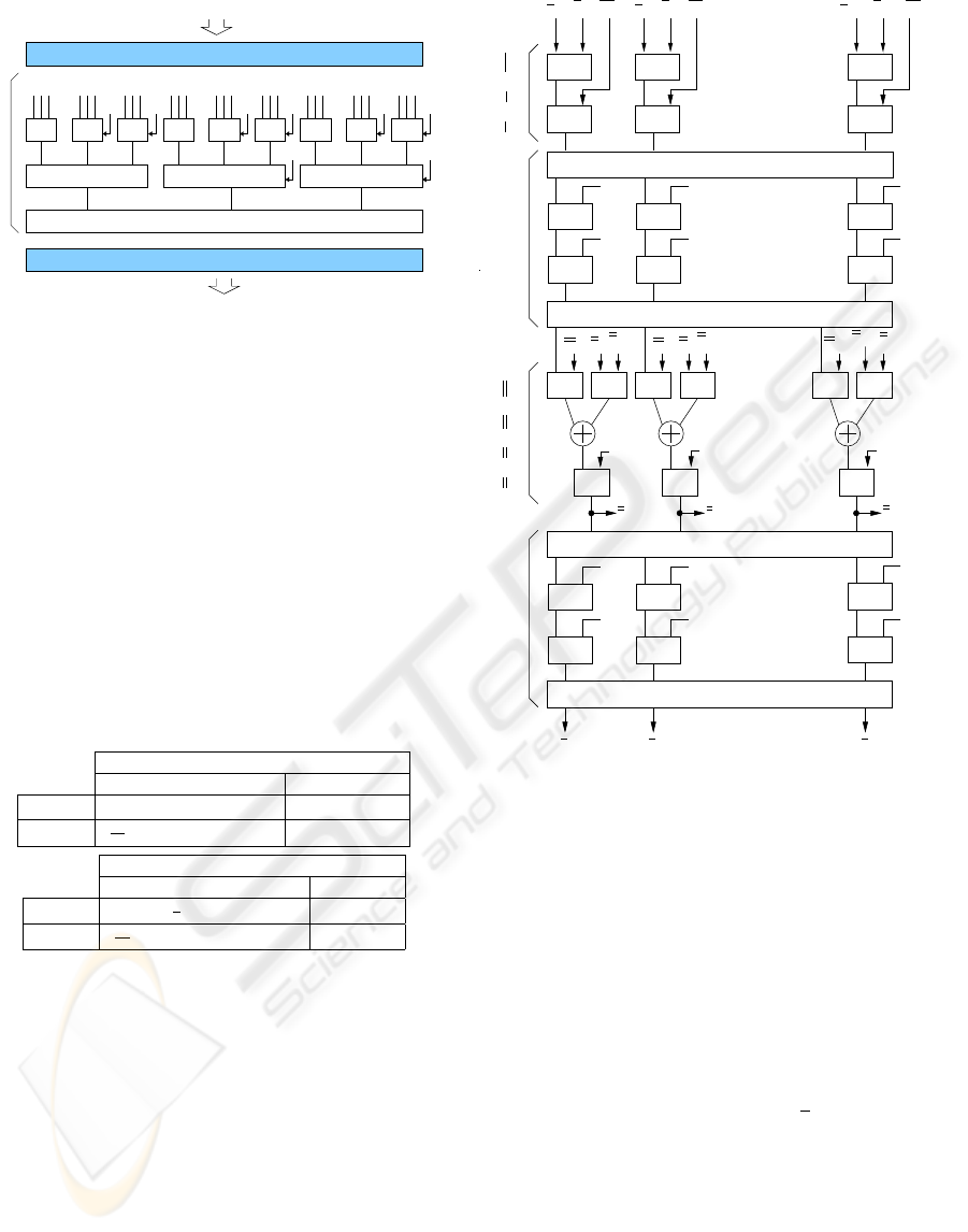
7 ARCHITECTURE AND
COMPLEXITY
We now present a hardware architecture associated to
Algorithm 3 in the special case where m
1
= t
2n
+t
n
+
1 and m
2
= t
2n/3
+t
n/3
+ 1. This choice enables us to
use the FFT circuit presented in the previous section.
The architecture of our binary field multiplier is given
in Figure 3. It is constituted of FFT blocks and multi-
pliers modulo m
1
(t) and m
2
(t).
Table 3: Complexity of multipliers modulo m
1
and m
2
.
Mul
m1
Space Time
#AND 3n
log
3
(6)
1
#XOR
72
5
n
log
3
(6)
−9n −7/5 3 log
3
(n) + 3
Mul
m2
Space Time
#AND
1
2
n
log
3
(6)
1
#XOR
36
15
n
log
3
(6)
−n/5 + n −1 3 log
3
(n)
These multipliers are referenced by blocks Mul
m
1
and Mul
m
2
in our architecture. Because of the special
form of m
1
(t) and m
2
(t) we can use the multiplier of
Fan and Hasan (Fan and Hasan, 2007) to perform this
operation. Therefore, the complexity (cf. Table 3) of
these blocks are easily deduced from (Fan and Hasan,
2007, Table 1).
The FFT blocks are designed using the ternary
method presented in previous section. Therefore,
their complexity are those given in (9) and (10). The
complexity of our multiplier can be evaluated with re-
spect to the numbers of each blocks and their cor-
responding space complexity denoted S , and time
complexity denoted D. For the space complex-
ity this gives 4nS (Mul
m
1
) + 5nS (Mul
m
2
) + 2S (FFT
m
1
) +
1
µ
−1
1
µ
−(n−1)
1
µ
n−1
1
µ
−(n−1)
2
a
1
m
0
1
b
1
b
n−1
a
n−1
FFT
m
1
b
1
a
1
m
1
b
1
a
0
m
0
b
n−1
m
n−1
a
n−1
µ
2
µ
n−1
2
1
1
1
µ
1
µ
−1
2
Mul
m
1
Mul
m
1
Mul
m
1
Mul
m
1
m
0
0
b
0
a
0
Mul
m
2
Mul
m
2
Mul
m
2
Mul
m
2
Mul
m
2
Mul
m
2
Mul
m
2
Mul
m
2
Mul
m
2
Mul
m
2
m
−1
1
Mul
m
1
Mul
m
1
Mul
m
1
Mul
m
1
Mul
m
1
Mul
m
1
Mul
m
2
A ×B ×M
0
convert
m
2
→m
1
FFT
m
1
m
0
n−1
r
0
r
1
r
n−1
FFT
m
2
FFT
m
2
Mul
m
2
Mul
m
2
Mul
m
2
Mul
m
1
Mul
m
2
Mul
m
2
Mul
m
1
r
0
r
1
r
n−1
m
−1
1
m
−1
1
(A ×B + Q ×M)m
−1
1
convert
m
1
→m
2
Figure 3: DPS-Lagrange Multiplier.
2S(FFT
m
2
) + 2n
2
/3 XOR. Similarly, the critical path
of this architecture gives the delay 4D(Mul
m
1
) +
4D(Mul
m
2
) + 2D(FFT
m
1
) + 2D(FFT
m
2
) + T
X
.
Using these expressions, (9),(10) and Table 3, we
can compute the complexity with respect to the num-
ber of XOR and AND gates and their corresponding
delay T
X
and T
A
.
Let r be the degree in t of the coefficients in
the DPS representation then deg
t
(m
2
) must satisfy
deg
t
(m
2
) ≥ r. Therefore, this implies that k ≤ r×n =
2n
2
/3 and thus leads to use n ≈
√
k, where k is the
degree of the field F
2
k
.
Finally, we obtain the complexity of the DPS-
Lagrange multiplier stated in Table 4. We also give in
this table the complexity of the best known method,
regarding space and time complexity, to perform bi-
nary field multiplication. One can remark that our ap-
proach decrease the space complexity from k
1.58
to
k
1.31
, while it is slower by a factor roughly equals to
5.3.
SUBQUADRATIC BINARY FIELD MULTIPLIER IN DOUBLE POLYNOMIAL SYSTEM
235

Table 4: Complexity comparison.
Space Complexity Time Complexity
Method # AND # XOR T
A
T
X
This paper 14.5k
1.31
69.6k
1.31
−31k + k
0.5
(8log
3
(k) + 39) 8 16log
3
(k) + 20
FH
∗
binary k
1.58
5.5k
1.58
−5k −0.5 1 2log
2
(k) + 1
FH
∗
ternary k
1.63
4.8k
1.63
−4k −0.8 1 3log
3
(k) + 1
FH
∗
= (Fan and Hasan, 2007);
8 CONCLUSION
In this paper we have presented a novel algorithm to
perform multiplication in binary field, using a Dou-
ble Polynomial System of representation. This system
enables the use of Fast Fourier Transform in the mul-
tiplication according to Lagrange representation. The
resulting multiplier still achieves a logarithmic time
complexity, but asymptotically improves the space
complexity from O(k
1.58
) to O(k
1.31
),
Our method is a first approach to reduce the space
complexity of binary field multiplier. In particular,
some optimizations can be done to reduce the con-
stant factors in the complexity. For example, a lot of
multiplications by a constant are counted as full mul-
tiplication in the current complexity evaluation.
Furthermore, one can also reduce the exponent
in the space complexity by replacing Fan and Hasan
multipliers with a quasi-linear approach (e.g. Schön-
hage’s technique (Schonhage, 1977)).
REFERENCES
Berlekamp, E. (1982). Bit-serial Reed-Solomon encoder.
IEEE Transactions on Inf. Th., IT-28.
Diffie, W. and Hellman, M. (1976). New directions in cryp-
tography. IEEE Transactions on Information Theory,
24:644–654.
Fan, H. and Dai, Y. (2005). Fast bit-parallel GF(2
n
) mul-
tiplier for all trinomials. IEEE Trans. on Comp.,
54(4):485–490.
Fan, H. and Hasan, A. (2007). A new approach to
subquadratic space complexity parallel multipliers
for extended binary fields. IEEE Trans. Comput.,
56(2):224–233.
Gao, S. (1993). Normal Bases over Finite Fields. Phd the-
sis, Waterloo University, Canada.
Gathen, J. v. and Gerhard, J. (1999). Modern Computer
Algebra. Cambridge University Press, New York, NY,
USA.
Giorgi, P., Jeannerod, C.-P., and Villard, G. (2003). On
the complexity of polynomial matrix computations.
In Proceedings of ISSAC’03, Philadelphia, Pennsyl-
vania, USA, pages 135–142. ACM Press.
Guajardjo, J. and Paar, C. (1997). Efficient algorithms for
elliptic curve cryptosystems. In Advances in Cryp-
tology, Proceedings of Eurocrypt’97, volume 1233 of
LNCS, pages 342–356. Springer-Verlag.
Hasan, M., Wang, M., and Bhargava, V. (1993). A Mod-
ified Massey-Omura Parallel Multiplier for a Class
of Finite Fields. IEEE Transactions on Computeurs,
42(10):1278–1280.
J.-C. Bajard, L.Imbert, T. P. (2005). Modular num-
ber systems: Beyong the mersenne family. In
SAC’04,Waterloo, Canada, volume 3357 of LNCS,
pages 159–169. Springer-Verlag.
Koblitz, N. (1987). Elliptic curve cryptosystems. Mathe-
matics of Computation, 48:203–209.
Mastrovito, E. (1991). VLSI architectures for computations
in Galois fields. PhD thesis, Dep.Elec.Eng.,Linkoping
Univ.
Miller, V. (1986). Use of elliptic curves in cryptogra-
phy. In Advances in Cryptology, proceeding’s of
CRYPTO’85, volume 218 of LNCS, pages 417–426.
Springer-Verlag.
Montgomery, P. L. (1985). Modular multiplication with-
out trial division. Mathematics of Computation,
44(170):519–521.
Mulders, T. and Storjohann, A. (2003). On lattice reduction
for polynomial matrices. Journal of Symbolic Compu-
tation, 35(4):377–401.
Schonhage, A. (1977). Schnelle multiplikation von poly-
nomen uber korpern der charakteristik 2. Acta Infor-
matica, 7:395–398.
Villard, G. (1996). Computing Popov and Hermite forms
of polynomial matrices. In Proceedings of ISSAC’96,
Zurich, Suisse, pages 250–258. ACM Press.
SECRYPT 2007 - International Conference on Security and Cryptography
236
