
BOUNDARY POINT DETECTION FOR ULTRASOUND IMAGE
SEGMENTATION USING GUMBEL DISTRIBUTIONS
Brian Booth and Xiaobo Li
Department of Computing Science, 2-21 Athabasca Hall, University of Alberta, Edmonton AB, Canada, T6G 2E8
Keywords:
Ultrasound Image Processing, Boundary Point Detection, Gumbel Distribution, log-Wiebull Distribution, A-
Mode Ultrasound, Data Fitting, Segmentation.
Abstract:
Due to high noise, low contrast, and other imaging artifacts, region boundaries in ultrasound images often do
not conform to the assumptions of many image processing algorithms. Specifically, the beliefs that region
boundaries have a high gradient magnitude or a high intensity can break down in this context.
In this paper, we present an alternative way of detecting likely boundary points in ultrasound images by
decomposing the image into one-dimensional intensity scans. These intensity scans, mimicking traditional
A-Mode ultrasound, are modeled using Gumbel distributions. Results show that the relationship between the
modes of these distributions and regions boundaries is relatively strong.
1 INTRODUCTION
Ultrasound image processing, particularly the task of
segmentation, has gained support in both the medical
and agricultural fields. In the medical field, computer
generated segmentation results are used to help diag-
nose heart disease as well as breast and prostate can-
cer (Noble and Boukerroui, 2006). Meanwhile, the
agricultural field uses segmentation results to deter-
mine the size of various cuts of meat in live animals.
Current image segmentation algorithms applied in
this field use assumptions about the appearance of a
region or its boundary that are common to general im-
age processing. One popular assumption used here is
that a region boundary is characterized by a strong
gradient. This is the foundation of many active con-
tour methods (Kass et al., 1987). Also popular is
the belief that a region boundary has a high intensity,
which has most notably been incorporated into Itti &
Koch’s saliency map algorithm and has a biological
basis (Itti and Koch, 2000). This assumption is of
particular interest in ultrasound image segmentation
as likely region boundaries tend to appear brighter in
ultrasound images than their surroundings (Middleton
et al., 2004).
Algorithms based on these two assumptions have
been used for ultrasound image segmentation with
some success. Gradient-based methods have achieved
good results on a limited subset of ultrasound im-
ages - particularly echocardiographs - where gradient
information is reliable boundary indicator (Yan and
Zhuang, 2003; Corsi et al., 2002). Intensity-based al-
gorithms have achieved mild success on both agricul-
tural and medical ultrasound images, but there is room
for improvement (Booth et al., 2006).
Unfortunately, these segmentation approaches are
limited due to the unique nature of ultrasound images.
These images are obtained in a different medium than
other real world images and have distinct types of
noise and imaging artifacts. Assumptions that have
held for the segmentation of other real world images,
particularly that regions boundaries have a high gra-
dient magnitude or high intensity, though appropriate
for some ultrasound images, generally do not hold.
As a result, it is important to return to the question:
What constitutes an edge in an ultrasound image?
In this paper, we present one approach for detect-
ing edge points in ultrasound images for the purpose
of segmentation. In this approach, a given ultrasound
image is decomposed into one-dimensional intensity
scans with the goal of replicating the original acous-
tical signals obtained by the ultrasound transducer as
179
Booth B. and Li X. (2007).
BOUNDARY POINT DETECTION FOR ULTRASOUND IMAGE SEGMENTATION USING GUMBEL DISTRIBUTIONS.
In Proceedings of the Second International Conference on Signal Processing and Multimedia Applications, pages 175-179
DOI: 10.5220/0002138701750179
Copyright
c
SciTePress
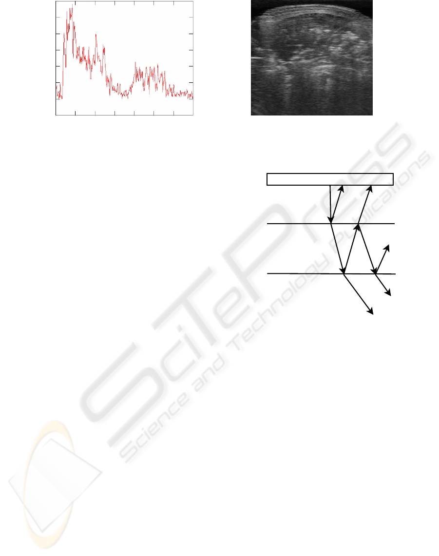
(a) A-Mode Ultrasound
(b) B-Mode Ultrasound
Figure 1: Ultrasound Imaging Types.
well as possible. These intensity scans are then mod-
eled as a probability distribution obtained from mul-
tiple independent Gumbel distributions, each distri-
bution representing a likely region boundary. Using
Expectation-Maximization, a predetermined number
of Gumbel density functions are fitted to each inten-
sity scan. The modes of the fitted distributions are
then taken as likely boundary points.
The algorithm was implemented and tested on 304
ultrasound images of in vivo pork loins and compared
with boundary point selection algorithms based solely
on intensity or gradient magnitude. Our results sug-
gest that there is a stronger relationship between the
modes of the fitted Gumbel distributions and region
boundary points than there is with the other two meth-
ods.
2 METHOD
To recognize the content of ultrasound images, it be-
comes important to understand the process through
which these images are formed. Therefore, a brief in-
troduction to the physics behind ultrasound imaging
is presented here prior to introducing the boundary
point detection algorithm.
2.1 Ultrasound Basics
The most common ultrasound imaging technique is
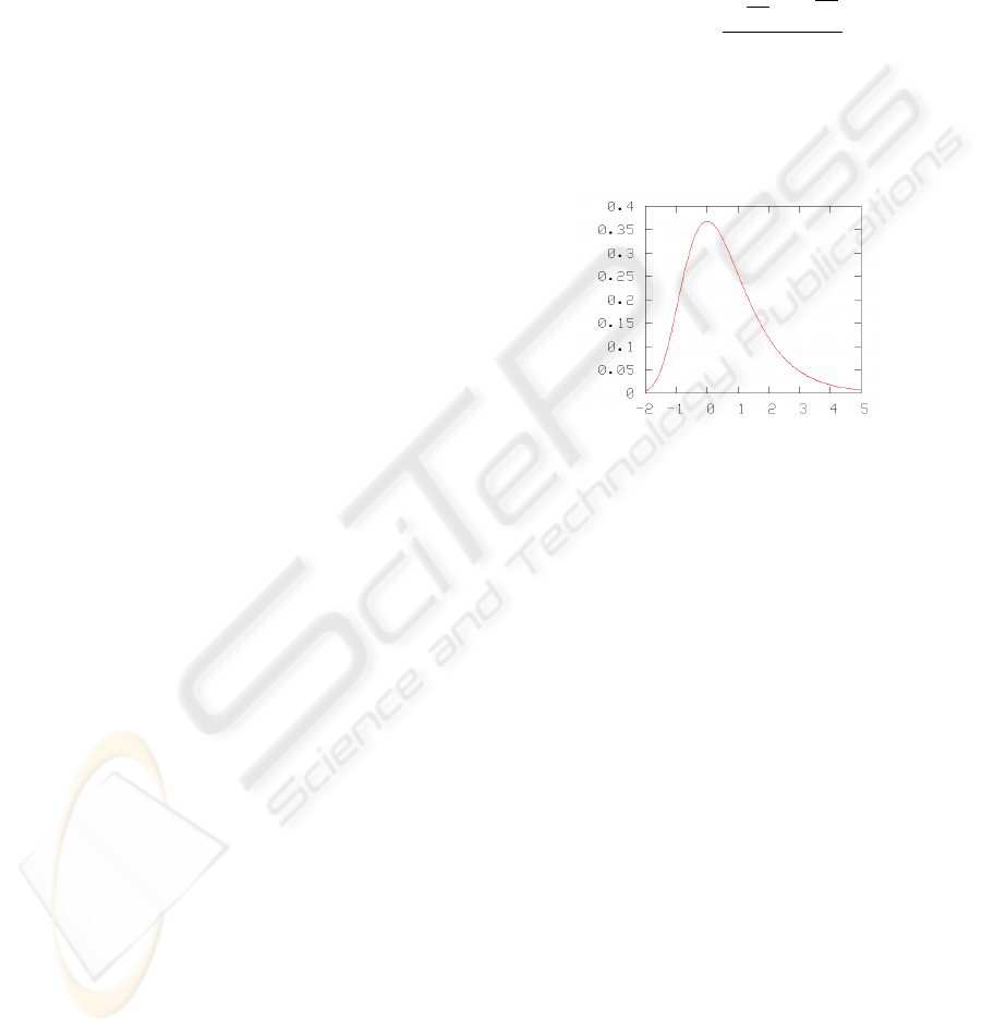
known as pulse-echo ultrasound. A simplified exam-
ple of this ultrasound technique is presented in Fig-
ure 2.
A single sound pulse, whose primary direction is
shown as T1, leaves the ultrasound transducer and
proceeds to enter the subject being scanned. As the
sound pulse continues outward, the density of the
medium through which the pulse travels will change.
This occurs most significantly at boundaries between
transducer
B1
B2
T1
T2
T2
T3
T4
T4
T3
T5
T5
Figure 2: The Reflection and Refraction of Sound Waves
from an Ultrasonic Scanner. As in (Muzzolini, 1996).
two tissues of different densities. When the pulse
reaches these types of acoustical boundaries, a portion
of the pulse reflects back towards the transducer while
a now weakened pulse refracts further into the sub-
ject. Once the reflected portion of the sound wave, re-
ferred to as an echo, returns to the transducer, its am-
plitude is recorded and using the formula distance =
2 ∗ velocity ∗ time, the depth at which the echo was
produced can be determined (Muzzolini, 1996).
Using a single transducer, the best we can do is
a one-dimensional scan known as an A-Mode (am-
plitude mode) scan. An example of such a scan is
presented in Figure 1(a). To create a two-dimensional
image, known as a B-Mode (brightness mode) scan,
an array of transducers are used. As a result, an ul-
trasound image is often considered as an array of A-
Mode ultrasound scans. An example of B-Mode ultra-
sound is shown in Figure 1(b). Pixel intensity in an ul-
trasound image corresponds directly to the amplitude
of the echoes received by the associated transducer.
In an ultrasound image, the transducer array can be
SIGMAP 2007 - International Conference on Signal Processing and Multimedia Applications
180
pictured as being at the top with each column of the
image representing an A-Mode ultrasound scan.
This form of image acquisition is susceptible to
noise for many reasons. First, most of our internal
tissues do not have a homogeneous density, result-
ing in echoes being recorded that are not near tissue
boundaries. The superposition of echoes that origi-
nated from different transducers also adds a particular
type of high intensity noise known as speckle noise.
However, the most problematic issue with ultrasound
in terms of noise is movement of the subject. Sim-
ply breathing can move tissue boundaries in ways that
distort the image (Middleton et al., 2004).
There are also many imaging artifacts common to
ultrasound, of which we mention two of particular in-
terest. First, note in Figure 2 that the strength of the
echoes recorded by the transducer will depend on the
angle at which the sound pulse meets a tissue bound-
ary. As a result, the amplitude of an echo, and in
turn the pixel intensity in an ultrasound image, will
be lower the less perpendicular a tissue boundary is to
the incident sound pulse.
Secondly, as an echo returns to the transducer, it
is common for a portion of the echo to reflect off the
transducer surface and reverberate between the trans-
ducer and the skin of the subject. This results is a
decay in amplitude after a strong echo is received in-
stead of a sharp drop-off (Muzzolini, 1996).
These two artifacts, combined with the amount of
noise common in ultrasound images, are the key rea-
sons why gradient magnitude and intensity may not,
on their own, be able to detect region boundaries. Fur-
thermore, the two imaging artifacts mentioned here
produce a distinctive pattern of echo responses for
a likely tissue boundary. In particular, the orienta-
tion dependence of the echoes results in a gradual rise
and fall in echo intensity around the depth of the tis-
sue boundary, while the reverberation of these echoes
leads to a decay in echo intensity following the tis-
sue boundary. This phenomenon can be seen in Fig-
ure 1(a).
2.2 Algorithm Description
The goal of the algorithm presented herein is to ob-
tain boundary points in ultrasound images by taking
advantage of the aforementioned physical properties
of ultrasound imaging. To achieve this goal, we de-
compose the given ultrasound images into its separate
columns and treat these columns as A-Mode ultra-
sound scans. Despite losing some spatial information
through this decomposition, we hope to gain an ad-
vantage by mimicking the original acoustical signal as
much as possible. Henceforth, we will be considering
one-dimensional scans similar to the one presented in
Figure 1(a).
By visual inspection, we note that the echo pat-
tern for a likely tissue boundary in an A-Mode scan
is similar in shape to the Gumbel probability distri-
bution, which is given by the following probability
density function:
f(x;µ, β) =
e
−
x−µ
β
e
−e
−
x−µ
β
β
(1)
The parameters, µ and β, represent the mode and
the spread of the density function respectively. A
graph of a sample Gumbel probability density func-
tion is presented in Figure 3.
Figure 3: A Sample Gumbel Distribution (µ = 0, β = 1).
Due to the similarities in shape, we model the in-
tensity distribution for the echoes from a potential
tissue boundary as a Gumbel distribution. An inde-
pendent collection of Gumbel distributions are fitted
to each A-Mode ultrasound scan using Expectation-
Maximization. Though it is clear that the echoes cre-
ated from deeper tissue boundaries are not indepen-
dent of the echoes from earlier tissue boundaries, the
intensity distributions from these echoes still retain
the same shape.
To use Expectation-Maximization, the number of
Gumbel distributions to fit to - and thereby the num-
ber of tissue boundaries in - each A-Mode scan must
be known ahead of time. The following algorithm is
used to estimate this number:
for i = 1:20,
- Fit a polynomial of degree i
to the A-Mode scan
- err[i] = average error between
the fitted polynomial and the
A-Mode scan
endfor
minDeg = i, where err[i] == min(err);
numGD = ceil(minDeg / 2);
Polynomials of various degrees are fitted to each
A-Mode scan using the Least Mean Squared algo-
BOUNDARY POINT DETECTION FOR ULTRASOUND IMAGE SEGMENTATION USING GUMBEL
DISTRIBUTIONS
181
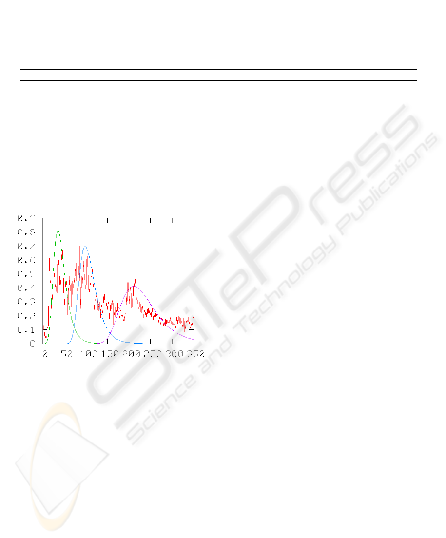
Table 1: Results for five different boundary point selection algorithms over 304 ultrasound images of in vivo pork loins.
Boundary Point Distance from Actual Boundary (in pixels) Percentage
Detection Algorithm Mean Std. Deviation Maximum Outliers
Gumbel Dist. Fitting 10.661± 2.329 7.356± 1.916 34.668± 8.661 87.768± 2.185
Intensity (equal number) 29.268± 8.844 27.823± 7.792 98.226± 23.406 87.270± 2.262
Gradient (equal number) 16.168± 5.964 15.374± 6.699 62.001± 23.034 88.837± 2.205
Intensity (top 13%) 3.922± 2.002 6.210± 3.235 28.209± 12.441 97.172± 0.252
Gradient (top 13%) 1.795± 0.581 2.155± 0.945 11.904± 4.891 97.350± 0.224
rithm. While these polynomials do not relate well
to the tissue boundaries represented in the scan, the
degree of the polynomial of best fit can be related to
the number of Gumbel distributions to fit to the scan.
The polynomial’s degree is divided by two on account
of the Gumbel distribution’s roughly parabolic shape.
An example of an A-Mode scan fitted with Gumbel
distributions is shown in Figure 4.
Figure 4: An A-Mode Scan Fitted with Three Gumbel Dis-
tributions. The Gumbel Distributions are Scaled for View-
ing Purposes.
The modes of the fitted Gumbel distributions are
taken as the most likely locations of the tissue bound-
aries the distributions represent.
3 EXPERIMENTAL RESULTS
The proposed boundary point detection algorithm was
implemented and tested on a set of 304 ultrasound
images of in vivo pork loins. The ultrasound im-
ages were recorded with an Aloka Flexus Model SSD-
1100 equipped with a 3.5MHz/127mm transducer Ul-
trasound system. The images are from between the
3rd and 4th ribs from the last rib and 7cm off the mid-
line of the pigs. This collection of images includes
the thirty-eight images used in (Booth et al., 2006).
For each image, we compare the detected bound-
ary points with a manually traced contour created
by an expert. The distance between each point on
the manually traced contour and the closest bound-
ary point is measured. The average, standard devia-
tion, and maximum values of these distances are cal-
culated for each image. Also calculated is the per-
centage of detected boundary points that are not the
closest boundary point for any of the points on the
manually traced contour.
The set of boundary points obtained by the pro-
posed algorithm are compared with those obtained by
thresholding based on intensity and gradient magni-
tude. Two thresholds are used: one which provides
an equal number of boundary points, and one that
gives thirteen percent of the image’s pixels as bound-
ary points. The second threshold is essentially the
same one used on intensity in (Booth et al., 2006).
Table 1 displays results for all five approaches.
Means and standard deviations for each measure are
provided over all images in the set.
Given an equal number of detected boundary
points, the intensity and gradient methods detect
points that have a much larger average distance to
the contour as well as a larger standard deviation than
the proposed approach, suggesting in those two cases
that large portions of the contour do not have any de-
tected boundary points nearby. Increasing the number
of likely boundary points in the intensity and gradi-
ent methods does seem to alleviate this problem, but
also introduces a significant amount of outliers, which
suggests that the relationship between those measures
and the contour are not as strong as with the proposed
algorithm.
Visual inspection appears to confirm that this is
in fact what is happening. Figure 5 shows the re-
sults from all five algorithms on an average case. De-
spite obvious outliers due to noise and other anatomi-
cal structures, boundary points are detected near large
portions of the contour using the presented approach.
SIGMAP 2007 - International Conference on Signal Processing and Multimedia Applications
182
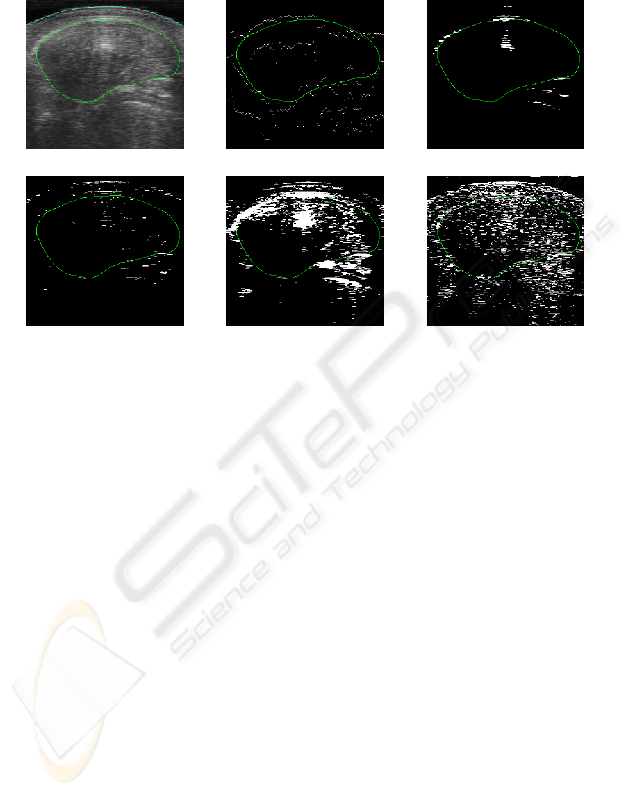
(a) Original Image with Contour
(b) Gumbel Distribution Fitting (c) Intensity (equal number)
(d) Gradient (equal number) (e) Intensity (13%)
(f) Gradient (13%)
Figure 5: Sample Boundary Point Detection Results from an Average Case for our Algorithm and Four Others. The Contour
is Displayed in Green while the Detected Boundary Points are Shown in White.
4 CONCLUSION
Given the different medium from which ultrasound
images are created, general assumptions about how
an edge is represented break down. Using knowledge
of how the images are acquired, we present a bound-
ary point detection algorithm that fits Gumbel dis-
tributions to mimicked A-Mode scans obtained from
an ultrasound image. Results on 304 in vivo pork
loin ultrasound images show that the relationship be-
tween the modes of the Gumbel distributions and ac-
tual boundary points is stronger than methods based
on other general image processing assumptions.
ACKNOWLEDGEMENTS
We gratefully acknowledge Dr. Alan Tong of La-
combe Research Centre, Agriculture and Agri-Food
Canada for providing the ultrasound image data for
this study. Also, thanks to the Natural Sciences and
Engineering Research Council of Canada (NSERC)
and the Informatics Circle of Research Excellence
(iCORE) for funding this project.
REFERENCES
Booth, B., Neighbour, R., and Li, X. (2006). On agricul-
tural ultrasound image segmentation. In Proceedings
of IEEE International Conference on Signal Process-
ing, pages 915–920.
Corsi, C., Saracino, G., Sarti, A., and Lamberti, C. (2002).
Left ventricular volume estimation for real-time three-
dimensional echocardiography. IEEE Transactions on
Medical Imaging, 21(9):1202–1208.
Itti, L. and Koch, C. (2000). A saliency-based search mech-
anism for overt and covert shifts of visual attention.
Vision Research, 40:1489–1506.
Kass, M., Witkin, A., and Terzopoulos, D. (1987). Snakes:
Active contour models. In Proceedings of the IEEE
International Conference on Computer Vision, pages
259–268.
Middleton, W. D., Kurtz, A. B., and Hertzberg, B. S. (2004).
Ultrasound, The Requisites, chapter Practical Physics,
pages 3–26. Mosby, Inc., 2 edition.
Muzzolini, R. E. (1996). A Volumetric Approach to Segmen-
tation and Texture Characterisation of Ultrasound Im-
ages. PhD thesis, University of Saskatchewan.
Noble, J. A. and Boukerroui, D. (2006). Ultrasound image
segmentation: A survey. IEEE Transactions on Medi-
cal Imaging, 25(8):987–1010.
Yan, J. Y. and Zhuang, T. (2003). Applying improved
fast marching method to endocardial boundary detec-
tion in echocardiographic images. Pattern Recogni-
tion Letters, 24(15):2777–2784.
BOUNDARY POINT DETECTION FOR ULTRASOUND IMAGE SEGMENTATION USING GUMBEL
DISTRIBUTIONS
183
