
FEATURES EXTRACTION FOR MUSIC NOTES RECOGNITION
USING HIDDEN MARKOV MODELS
Fco. Javier Salcedo, Jesús Díaz-Verdejo and José Carlos Segura
Department of Signal Theory, Telematics and Communications, Granada University, Spain
Keywords: Music information retrieval, Hidden Markov Models, music features extraction, music notes recognition.
Abstract: In recent years Hidden Markov Models (HMMs) have been successfully applied to human speech
recognition. The present article proves that this technique is also valid to detect musical characteristics, for
example: musical notes. However, any recognition system needs to get a suitable set of parameters, that is, a
reduced set of magnitudes that represent the outstanding aspects to classify an entity. This paper shows how
a suitable parameterisation and adequate HMMs topology make a robust recognition system of musical
notes. At the same time, the way to extract parameters can be used in other recognition technologies applied
to music.
1 INTRODUCTION
The music represents another way in human
communication. Instead of transmitting ideas like in
voice, they express (or they try to express) feelings
(Scheirer, E. D., 2000). At this moment, techniques
and systems of speech recognition are in a more
developed stage than its equivalents for music. The
reasons are simple: the complexity of the music
signal due to the variety of the possible sounds, and
its structure in several and simultaneous levels:
polyphony (De Pedro, D., 1992). That leads to
unsatisfactory results obtained by the recognition
systems when they are applied to music. On the
other hand, Hidden Markov Models (HMMs) have
shown good performances when applied to human
speech recognition, making them suitable for real
applications. We will show in this work that, with an
adequate parameterisation, and the incorporation of
information about the musical structure, HMMs can
also be successfully employed for music.
There are few specific works described in the
bibliography that make a study of the best-suited
parameters to characterize the musical signal. The
first studies tried to extract the pitch of the signal in
order to detect the music notes like Kashino’s
(Kashino, K., Murase, H., 1998) and Gómez’s works
(Gómez, E., Klapuri, A., Meudic, B., 2003). One of
the most outstanding is Beth Logan’s work (Logan,
B., 2000). She shows that cepstral coefficients are
appropriate for discriminating between music and
voice. She finally points out the need to accomplish
a deeper study about the quantity of coefficients
used, the sampling period, the size of the windows
and the perceptual scale, in order to model the music
efficiently. In another work, Durey and Clements,
use the HMMs to index music by melody (Durey,
A.S., Clements, M.A., 2001 and 2002). They make a
soft study to determine the best features to use for
music. This study is made using the FFT (Fast
Fourier Transform) coefficients, the Log Mel-scale
filter bank parameters and the MFCCs (Mel
Frequency Cepstral Coefficients). The best results
were obtained by MFCCs. Unfortunately Durey did
not justify other values used in the parameterisation,
like the size of the windows or the number of
coefficients chosen.
The present paper has a clear objective: to
determine a suitable parameterisation for musical
signals. The article begins (Section 2) with a simple
explanation about the musical notes and the basic
foundations of HMMs. Section 4 is devoted to some
basics of the HMMs (topology, training and
grammar) used in the recognition system. After that,
in Section 4 the database used to develop and test
the system is described, while Section 5 shows some
details of the implemented recognition system. From
this point, the sequence of experiments to determine
the best parameterisation is described. The system is
tested in two conditions: with pieces of music played
with one instrument (Section 6), and later with the
same pieces played with other different instruments
184
Javier Salcedo F., Díaz-Verdejo J. and Carlos Segura J. (2007).
FEATURES EXTRACTION FOR MUSIC NOTES RECOGNITION USING HIDDEN MARKOV MODELS.
In Proceedings of the Second International Conference on Signal Processing and Multimedia Applications, pages 180-187
DOI: 10.5220/0002139301800187
Copyright
c
SciTePress
(Section 7). The results obtained by the proposed
recognition system are compared with those
provided by Durey’s system on the same database
when using the best parameters. Finally, the last
section offers conclusions.
2 THE MUSICAL NOTES
A musical note is completely characterized by four
values (Seguí, S., 1984):
1. Name: The name of the musical note determines
its height or frequency within the musical scale.
There are seven names for musical notes from A
to G.
2. Musical scale: The general scale of the sounds
includes all the range of sounds inside the limits
of identification for the human ear.
Approximately such limits are between 27 and
4750 Hz, which match with the lowest and the
highest note played by a concert piano,
respectively. The general scale is divided into
sets, named octaves. Each octave has a number
to indicate the position in the general scale,
which is called the acoustic index.
3. Alteration: The tone is the distance between two
notes without alteration. There are two
exceptions, the first one, between the E and F
notes and the second between the B and C notes
in the same scale. A note can be changed in one
of two directions:
• Sharp. The intonation of the affected sound
increases one semitone.
• Flat. Reduce one semitone the intonation of
the affected sound.
Therefore, the note name, its octave, and if there is a
change or not, determines the fundamental
frequency of the musical note.
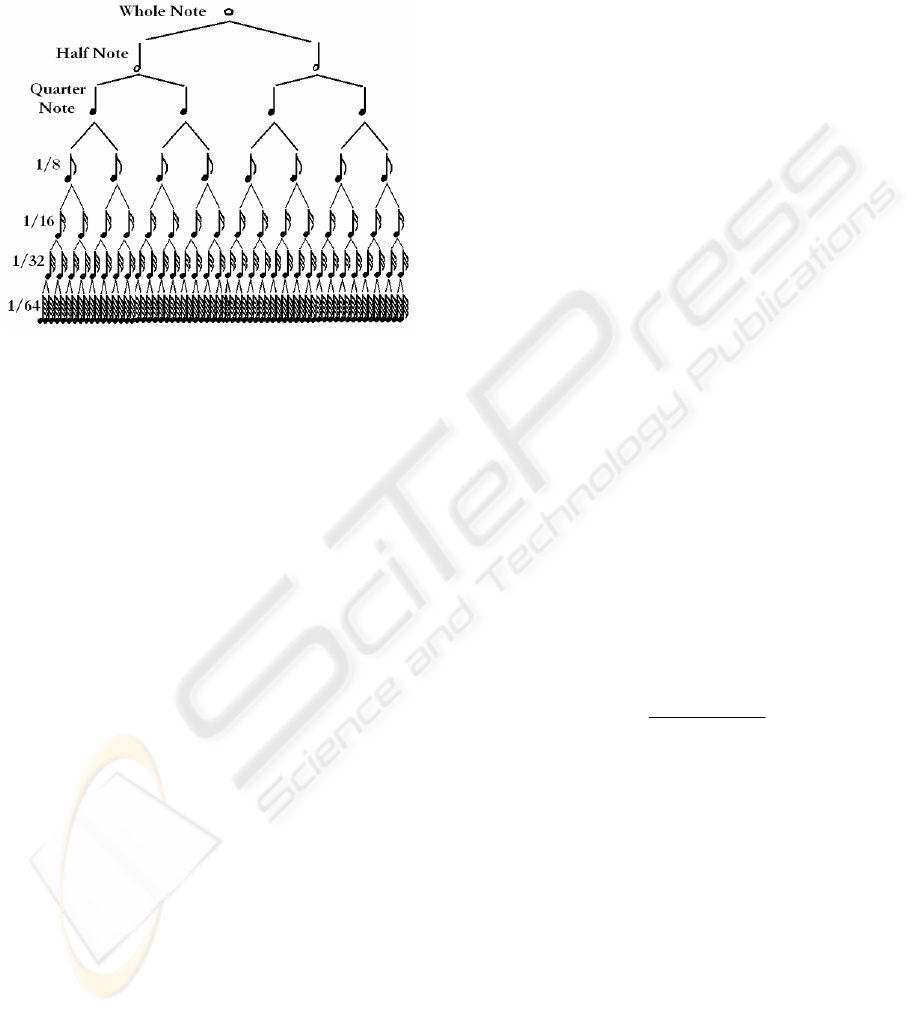
4. Duration: The duration of the notes are defined
in a relative way. The relation between two
adjacent notes duration is a half time. The
longest duration note is the whole note. The
next one is the half note which is played in a
half time of the whole note and so on. This
partition time process continues until it’s
obtained the shortest note, the sixty-fourth note
(Figure 1).
3 RECOGNITION SYSTEMS
BASED ON HMMS
These kinds of recognition systems are characterized
by the use of a production model, that is, by a
Hidden Markov Model. These production models
are estimated through a training phase, in which
enough patterns have to be offered to the system.
The recognition procedure can be described as
the calculation of the probabilities P(W|O) that an
observation O is produced by some model or
sequence of models W, on all the set of possible
models, in order to find the one that provides the
maximum value,
ˆ
W
.
{P(W|O)}
i
|O)WP( max=
∧
(1)
Probabilities P(W|O) cannot be directly
evaluated, but they can be obtained using Bayes's
rule according to:
P(O)
P(O|W)P(W)
P(W|O)
⋅
=
(2)
where the
P(W) is the “a priori” probability of the
model or the sequence of models
W, P(O|W) is the
production probability to observe
O given the
sequence of models
W, and P(O) the probability that
the observation
O takes place. We can suppose P(O)
constant for a given input. Then, the task of
recognition implies finding the model, or the set of
models, that maximizes the product
P(W)·P(O|W)
instead of P(W|O). In this way, in our case, it is
necessary to consider two models: the acoustic
model, determined by
P(O|W), and the language
model, described by “a priori” probabilities P(W).
The acoustic model can be represented by using
Hidden Markov Models (Rabiner, L., Juang, B.,
Levinson, S., Sondhi, M., 1985), while the language
Figure 1: Relations between note durations.
FEATURES EXTRACTION FOR MUSIC NOTES RECOGNITION USING HIDDEN MARKOV MODELS
185
model can be modelled by a probabilistic finite state
automaton.
The recognition unit used is the note, which is
modelled through HMMs. This way, each HMM
will represent a single note, while the language
model or grammar contains information about valid
sequences of notes. This is possible through the
inclusion of a probability of such sequences.
The constituent elements of a Hidden Markov
Model are five (Rabiner, L., 1989):
1. A set of
N interconnected states, which must be
reachable from at least one state.
},...,s,s,s{sS
N321
=
(3)
2. A set of M observable symbols that can be
produced by HMMs.
},...,o,o,o{oO
M321
=
(4)
3. A matrix of transition probabilities between
states,
A={a
ij
}. This is a square matrix of
dimension N. Each element a
ij
corresponds to
the transition probability from the state
s
i
to the
state s
j
. The values of a
ij
elements must be
between 0 and 1, due to its probabilistic nature.
Transition probabilities with the same origin
state must be normalized:
1a
1
ij
=
∑
=
N
j
(5)
4. A set of parameters
B={b
i
(k)} that define for
each state the probability density function of
productions. Assuming that
x
t
represents the
observation value at instant t, each b
i
can be
defined according to:
Ni) so|qP(x(o)b
itti
≤≤
=
=
=
1
(6)
5. A set of initial-state probabilities
P={π
i
}, where
π
i
is the probability that HMM starts on state s
i
:
Ni) sP(qπ
ii
≤≤== 1
1
(7)
The initial-state transitions probabilities
π
i
should
verify:
1
1
=
∑
=
N
i
i
π
(8)
4 THE MUSIC DATABASE
One of the problems that arises in recognition
systems is how to offer enough well identified
samples to them. Thus, the database must contain
enough notes of each type in this case. On the other
hand, all the notes must be identified in the signal
correctly, that is, to set the name of the note played,
and the period of time that note appears on the
signal. This is called the labelling process. We have
chosen MIDI format because it offers the possibility
to generate note sequences and to label the musical
signal automatically. The process to make the
database is the following: the MIDI samples with
0
1000
2000
3000
4000
5000
6000
7000
8000
9000
A3 B3 C3 D3 E3 F3 G3 A4 B4 C4 D4 E4 F4 G4 A5 B5 C5 D5 E5 F5 G5 sil
Appearance frequency
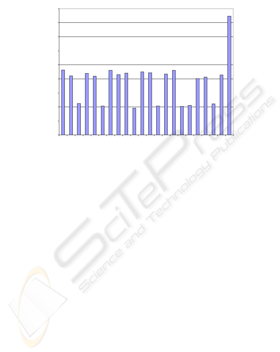
Figure 2: Statistical appearances of the notes in all the database samples.
SIGMAP 2007 - International Conference on Signal Processing and Multimedia Applications
186
aleatory note sequences are generated first, then they
are played and recorded using some instruments as
live music to obtain the database samples. The
recognition system is trained and tested using these
samples. Finally the labelling process is applied
using the information contained in the original MIDI
samples.
The database is made with 100 MIDI samples of
30 seconds. Each sample is a sequence of aleatory
notes and silences of the same duration (180 ms).
These MIDI samples have been recorded using five
instruments: piano, guitar, clarinet, organ and
vibraphone. Then 500 samples are obtained in single
channel wav format.
The signals have been generated in MIDI format
using aleatory notes. In this way, there is the same
probability for all the possible note sequences. This
fact lets the recognition system focus on the acoustic
model improvement, instead of the language model,
that will be affected using real music.
The musical notes from the samples belong to
the scales with index 3, 4 and 5, that is, attending to
its fundamental frequencies, from 132 to 1056 Hz.
There aren’t any altered notes (flats or sharps) in
database samples. Figure 2 shows the statistical
appearances of the notes and the silence in all the
samples of the database. It can be observed that
there are three different appearance frequencies.
This fact allows to know if the training stage is made
correctly, when there is no significant recognition
results between notes with different appearance
frequencies.
5 THE NOTES RECOGNITION
SYSTEM
Some parameters and properties of the recognition
system need to be established before exposing the
parameterisation study.
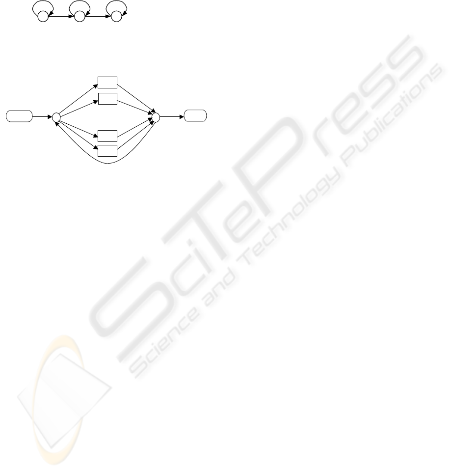
5.1 HMMs Topology
The temporary evolution of a musical note can be
split into three parts (Fletcher, N. H., Rossing, T. D.,
1991): the attack, sustain and relaxation zone. This
fact suggests using a HMM model for each note with
three states. Each of these states will model one of
the three zones of a musical note. The model is a
Bakis’s one, so there are only forward transitions
between one state and the next, and self-transitions
(Figure 3).
5.2 Grammar
The grammar, according to the sampled database,
consists in an undetermined succession of notes that
have the same probability of taking place in the
sequence. The notes that can appear in the musical
signal belong to scales 3, 4 and 5. Therefore there
are 21 different notes plus silence, which makes 22
symbols. Figure 4 shows the grammar used, which
allows transitions between all the notes and the
silence.
5.3 Training
The models are started by extracting all the
realizations of each note from the training set. For
this purpose it is necessary to consider the
segmentation derived from the labelling of the
recorded samples Later, Baum-Welch's algorithm
(Rabiner, L., 1989) is used for isolated training of
HMMs. The number of training iterations have been
adjusted to get differences below 10
-5
in log(P(O|λ))
between two successive training iterations.
In order to improve the statistical validity of the
results the Leave-one-out method has been used. We
have chosen 80% of the samples for training and the
other 20% for recognition purposes. This way 5
partitions of the database samples have been
established. In each experiment, 4 of them are used
for training and the last one for recognition.
1 2 3
States
Figure 3: HMMs topology to detect musical notes.
START
END
A
3
B
3
sil
G
5
. . .
Figure 4: Grammar used for note recognition. The initial
and final confluence points enable any sequence of notes
and silences.
FEATURES EXTRACTION FOR MUSIC NOTES RECOGNITION USING HIDDEN MARKOV MODELS
187

6 PARAMETERISATION
FOR UNIQUE INSTRUMENT
RECOGNITION
This experiment tries to obtain an initial
parameterisation for mono-instrumental recognition
conditions. For this reason the system is to train and
to evaluate using only the piano samples of the
database.
6.1 Initial Parameterisation
The initial parameterisation used is based on
Logan’s study (Logan, B., 2000) and the one used
by the authors on rhythm detection (Salcedo, F.J.,
Díaz, J.E., Segura, J.C., 2003). The way the features
are extracted is done in the following way:
1. The recordings were made at a sampling rate of
22050 Hz using a single channel.
2. Hamming windows are applied over the signal
to extract the features vectors. The windows
have a 15 ms size and are overlapped by 50% of
its size: 7.5 ms.
3. For each window the first 14 MFCCs (Mel
Frequency Cepstral Coefficients) and the energy
are calculated. The first and second order
coefficients are calculated too. This makes an
amount of 45 coefficients for each characteristic
vector.
4. Parameters have been extracted making an
energy normalization in the samples in order to
minimize undesirable effects caused by
different recording conditions.
6.2 Signal filtering
The signals to be used by the system must be filtered
according to a bandwidth. We have selected three
bandwidths to evaluate. These bandwidths
correspond to different configurations of complete
scales and the harmonic zone. Bearing in mind that
the musical notes of the samples belong to the scales
3, 4 and 5, the filtering bands to evaluate are the
following:
• The scales that belongs to the notes of the
samples, that is, from 128 to 1023 Hz.
• The scales 3, 4 and 5, and all the highest scales
including the harmonics zone to 8184 Hz.
• All the possible scales and the harmonic zone
from 64 to 8,184 Hz.
The filtering limits are calculated as the half-way
frequency between the last note of the previous scale
and the first one belonging to the following scale.
6.3 Number of Mel filters
Another parameter under consideration is the
number of Mel filters, that in all cases have been
taken equal to the number the notes present in the
filtering bandwidth, or in sequences like:
1k 1)1(2
1
≥−+=
−
MF
k
(9)
where the F is the number of filters, and M is the
number of notes that exists in the considered
bandwidth. This way, the number of filters is
proportional to the number of musical notes of the
considered band.
Table 1: Recognition and error rates varying filter bandwidth and the number of filters in Mel scale (piano samples).
Filtering (Hz) Number of
filters
% correct
notes
% deleted
notes
% substituted
notes
% inserted
notes
Percent
Accuracy
64-8.184 49 97,66 0,60 1,74 1,20 96,46
128-8.184 35 98,73 0,67 0,60 1,28 97,45
128-8.184 71 97,49 0,59 1,92 0,98 96,51
128-1.023 21 98,77 1,22 0,01 1,54 97,23
128-1.023 43 99,02 0,95 0,03 1,73 97,30
128-1.023 87 99,17 0,82 0,01 1,09 98,08
128-1.023 175 99,12 0,82 0,07 1,76 97,37
Table 2: Comparison between Durey’s system and the best results obtained in the experiment with one instrument.
SYSTEM
% Correct
notes
% deleted
notes
% substituted
notes
% inserted
notes
Percent Accuracy
Durey 86,73 11,31 1,97 4,81 81,92
Best features
99,17 0,82 0,01 1,09 98,08
SIGMAP 2007 - International Conference on Signal Processing and Multimedia Applications
188

6.4 Results
Table 1 shows the different precision accuracies
(PAs) and error rates obtained by the system with
various filtering bandwidths and number of filters in
Mel scale. The best results are obtained applying the
bandwidth corresponding to the fundamental
frequencies of the notes, and by using 87 filters.
Thus the optimum number of filters is obtained from
expression (9) with
k=3.
This result is 16% better in precision accuracy
than that obtained by Durey’s system using the same
samples database (Table 2). The improvements
observed for the developed system are due not only
to the features extraction, but also by other aspects
like HMMs topology.
7 FEATURES FOR
MULTI-INSTRUMENTAL
NOTES RECOGNITION
This experiment is aimed at obtaining an improved
parameterisation for multi-instrumental notes
recognition.
This experiment is affected by a high number of
variables. Thus, in order to make the diagnosis
results easier, and to decrease the number of possible
combinations, it has been carried out in three stages:
• First: In this stage we try to determine the cut-
off filtering frequencies and the number of
filters applied in Mel scale. The variables in this
phase are the same as the ones used in the
previous experiment.
• Second: This stage attempts to find the number
of MFCC coefficients necessary to characterize
musical notes adequately.
• Third: It is the final stage in which the size of
the windows and their overlay are evaluated.
7.1 First Stage
Results are worse than those obtained in previous
experiments using the best parameterisation (Table
3). Now, the percentage accuracy has decreased to
77.02%, using the 128-1023Hz bandwidth, and 87
filters. The introduction of new instruments has
triggered the error rates, as we could expect.
Nevertheless, we can extract a conclusion from
the data shown in Table 3: the system obtains the
best results with bigger bandwidths, because the best
PAs of the series surpass 80%. Therefore it’s better
to use a method of filtering in which all the possible
scales and the harmonics zone are included, that is
the 64 to 8.184Hz bandwidth.
Insertion errors descend to the minimum value
using 99 filters, while deletion and substitution
errors are also one of the best from the table.
Therefore, the optimum filters number is the one
obtained from expression (9) with the value
k=2.
Comparing the best results obtained until now
with Durey's system evidences that the proposed
system improves by 10% the accuracy rate.
Nevertheless, we observe less success in detecting
notes, because substitution errors are greater than in
Durey’s one.
7.2 Second Stage
This phase is aimed at knowing how many MFCC
coefficients are needed in order to get more
information from the music signal.
At first sight, the results exposed in Table 4 have
higher PA (10%) than those obtained in the previous
stage. On the other hand, substitution errors decrease
appreciably when the coefficient number is higher.
The rest of the error rates are around the same levels,
and even increase a little. We can see a saturation for
the accuracy rate when up to 35 coefficients are
used.
Table 3: Recognition and error rates varying filter bandwidth and the number of filters in Mel scale. The notes of the
samples are interpreted by various instruments.
Filtering (Hz) Number of
filters
% correct
notes
% deleted
notes
% substituted
notes
% inserted
notes
Percent
Accuracy
128-1.023 21 83,25 2,10 14,65 7,08 76,18
128-1.023 43 85,15 2,32 12,53 5,45 79,70
128-1.023 87 82,80 2,73 14,47 5,79 77,02
128-8.184 35 82,03 1,41 16,56 12,37 69,66
128-8.184 71 82,67 1,47 15,86 6,55 76,13
128-8.184 143 81,97 1,61 16,42 5,67 76,30
64-8.184 49 84,82 1,77 13,41 4,05 80,77
64-8.184 99 85,16 1,96 12,88 3,79 81,37
FEATURES EXTRACTION FOR MUSIC NOTES RECOGNITION USING HIDDEN MARKOV MODELS
189

Although at this point there are more indications to
use 35 MFCCs to characterize the music signal, we
chose 40 for two reasons:
1. To make sure that the parameterisation of the
system is within the saturation zone of
information provided by the MFCCs.
2. Although this number of coefficients doesn’t
provide the best accuracy rate, it is the one that
gets minor substitution errors. This kind of error
goes down significantly by increasing the
MFCCs number.
7.3 Third Stage
It’s possible that the high insertion rates of the
system at this point, could be given by the different
temporary evolution of the notes played with
different instruments. This fact motivates the
following system tests, which consists of using
several window sizes with some different overlays
between them.
The window sizes used in the experiment
oscillate between 30 and 90 ms with overlays
between 50 and 80% of the window size.
Table 5 shows the experimental results. The
optimum point is produced using 60 ms windows
displaced by 12 ms. On the other hand, the
successful outcome of the results confirms the
validity of the HMMs topology for notes
recognition.
Figure 5 represents the percentage accuracy
evolution of the recognition system through the
successive parameterisation improvements made in
experiments.
Finally, we have to point out that accuracy rate
obtained by Durey’s system is 71.7% in multi-
instrument recognition conditions. This value is
lower than any one obtained by the proposed system
in any experiment in all the three stages (Table 5).
8 CONCLUSIONS
The present work shows a study on a suitable set of
features extracted from the signal to be used in
musical notes recognition. Likewise, Hidden
Markov Models have been shown to be powerful
enough when applied to musical notes recognition.
Table 4: Recognition and error rates varying the number of MFCCs.
Number of
MFCCs
% correct
notes
% deleted
notes
% substituted
notes
% inserted
notes
Percent Accuracy
14 85,16 1,96 12,88 3,79 81,37
20 92,49 1,75 5,77 4,29 88,19
25 95,14 1,50 3,36 4,66 90,48
30 96,72 1,70 1,58 4,73 91,99
35 97,39 1,97 0,64 4,93 92,46
40 97,43 2,10 0,46 5,84 91,60
45 97,27 2,18 0,55 6,05 91,22
Table 5: Recognition and error rates varying the windows width and its overlapping.
Window
Width (ms)
Overlapping
(ms)
% correct
notes
% deleted
notes
% substituted
notes
% inserted
notes
Percent
Accuracy
30 6 98,23 1,55 0,22 4,95 93,28
30 7,5 98,29 1,54 0,17 6,86 91,43
30 10 98,16 1,62 0,22 8,31 89,85
30 15 96,49 3,12 0,39 3,59 92,97
60 12 98,43 1,25 0,32 0,17 98,26
60 15 98,11 1,65 0,24 0,05 98,06
60 20 97,16 2,61 0,23 0,01 97,15
60 30 95,94 3,63 0,42 0 95,95
90 18 97,90 1,91 0,19 0,04 97,86
90 22 97,10 2,65 0,25 0 97,10
90 30 96,10 3,61 0,30 0,01 96,08
90 45 94,14 5,49 0,37 0 94,14
SIGMAP 2007 - International Conference on Signal Processing and Multimedia Applications
190

A suitable parameterisation and adequate models
have led to a robust basic recognition of musical
notes in cases of multi-instrumental recognition
conditions.
Finally, it is necessary to point out that the
parameterisation obtained can be used in other
recognition technologies.
REFERENCES
De Pedro, D., 1992. Teoría Completa de la Música.
Editorial Real Musical.
Durey, A.S., Clements, M.A., 2001. Melody Spotting
Using Hidden Markov Models. In Proceedings of
ISMIR 2001, International Symposium on Music
Information Retrieval.
Durey, A.S., Clements, M.A., 2002. Features for Melody
Spotting Using Hidden Markov Models. In
Proceedings of ICASSP 2002, International
Conference of Acoustic Signal and Speech Processing.
Fletcher, N. H., Rossing, T. D., 1991. The Physics of
Musical Instruments. Springer-Verlag, New York,
1991.
Logan, B., 2000. Mel Frequency Cepstral Coefficients for
Music Modelling. In Proceedings of ISMIR 2000,
International Symposium on Music Information
Retrieval.
Kashino, K., Murase, H., 1998. Music Recognition Using
Note Transition Context. In Proceedings ICASSP, pp.
VI 3593–6.
Gómez, E., Klapuri, A., Meudic, B., 2003. Melody
Description and Extraction in the Context of Music
Content Processing. Journal of New Music Research.
Volume 32, Number 1, March 2003.
Rabiner, L., Juang, B., Levinson, S., Sondhi, M., 1985.
Recognition of Isolated Digits Using Hidden Markov
Models with Continuous Mixture Densities. AT&T
Tech Journal.
Rabiner, L., 1989. A Tutorial on Hidden Markov Models
and Selected Applications in Speech Recognition.
Proceedings of the IEEE 1989.
Salcedo, F.J., Díaz, J.E., Segura, J.C., 2003. Musical Style
Recognition by Detection of Compass. In Proceedings
of IBPRIA 2003 Iberian Conference on Pattern
Recognition and Image Analysis.
Scheirer, E. D., 2000. Music-Listening Systems. Doctoral
thesis, Massachusetts Institute of Technology.
Seguí, S., 1984. Curso de Solfeo. Editorial Unión Musical
Española.
75
80
85
90
95
100
One
instrument
64-8184Hz
filtering
More filters More MFCCs 60ms
windows
Percent Accuracy (%)
Figure 5: Percent accuracy evolution of the system from the initial parameterisation to the last stage.
Table 6: Comparison between Durey’s system and the best results obtained in the experiment with multiple instruments.
SYSTEM % Correct
notes
% deleted
notes
% substituted
notes
% inserted
notes
Percent Accuracy
Durey 81,71 10,71 7,57 10,01 71,70
Best features 98,11 1,65 0,24 0,05 98,06
FEATURES EXTRACTION FOR MUSIC NOTES RECOGNITION USING HIDDEN MARKOV MODELS
191
