
EXPLANATION GENERATION IN
BUSINESS PERFORMANCE MODELS
With a Case Study in Competition Benchmarking
Hennie Daniels
1,2
and Emiel Caron
2
1
Center for Economic Research, Tilburg University, P.O. Box 90153, 5000 LE, Tilburg, The Netherlands
2
Erasmus Research Institute of Management (ERIM), Erasmus University
P.O. Box 90153, 3000 DR, Rotterdam, The Netherlands
Keywords:
Decision Support Systems, Finance, Production Statistics, Artificial Intelligence, Explanation.
Abstract:
In this paper, we describe an extension of the methodology for explanation generation in financial knowledge-
based systems. This offers the possibility to automatically generate diagnostics to support business decision
tasks. The central goal is the identification of specific knowledge structures and reasoning methods required
to construct computerized explanations from financial data and models. A multi-step look-ahead algorithm is
proposed that deals with so-called cancelling-out effects. The extended methodology was tested on a case-
study conducted for Statistics Netherlands involving the comparison of financial figures of firms in the Dutch
retail branch. The analysis is performed with a diagnostic software application which implements our theory
of explanation. Comparison of results of the method described in (Daniels and Feelders, 2001) with the results
of the extended method clearly improves the analyses when cancelling-out effects are present in the data.
1 INTRODUCTION
Competition benchmarking or interfirm comparison
(IFC) is defined as the regular measuring and com-
paring of a company’s performance against its com-
petitors, against industry leaders or industry and his-
toric averages. The aim is often to learn how the com-
pany can improve its own performance. By compar-
ing the financial variables of a company with those
of other companies, the company can assess its per-
formance against objective standards and see where
the company is strong or weak. Currently, the diag-
nostic process for IFC is mostly carried out manually
by business analysts (a.o. bankers, accountants and
consultants). The analyst has to explore large data
sets in the domain of business and finance to spot
firms that expose exceptional behaviour compared to
some norm behaviour. After abnormal behaviour is
detected the analyst wants to find the causes, the set of
financial variables responsible, that explain the firm’s
behaviour. Today’s information systems for auto-
mated financial diagnosis and interfirm comparison
have little explanation or diagnostic capabilities. Such
functionality can be provided by extending these sys-
tems with an explanation formalism, which mimics
the work of human analysts in diagnostic processes.
In this paper the diagnostic process is fully automated
and implemented in a computer program to support
decision-makers.
Diagnosis is generally defined as finding the best
explanation of observed symptoms of a system under
study. This definition assumes that we know which
behaviour we may expect from a correctly working
system. Diagnosis of business performance is defined
as explaining the difference between the actual perfor-
mance of a company and its norm performance. The
norm performance or normative model can be derived
from some statistical model or can be expert knowl-
edge from financial analysts. Two important consecu-
tive phases in a diagnostic process are problem identi-
fication (or symptom detection) and explanation gen-
eration (Verkooijen, 1993). When a discrepancy be-
tween actual and norm behaviour is discovered, and
is qualified as exceptional with respect to some speci-
fied norm, the next step is to explain this discrepancy
using our “understanding” of the system. There are
many contributions on medical diagnosis and diagno-
sis of technical devices, see (Verkooijen, 1993) for
an overview. A limited number of approaches have
been proposed for the automatic generation of expla-
119
Daniels H. and Caron E. (2007).
EXPLANATION GENERATION IN BUSINESS PERFORMANCE MODELS - With a Case Study in Competition Benchmarking.
In Proceedings of the Ninth International Conference on Enterprise Information Systems - AIDSS, pages 119-128
DOI: 10.5220/0002346101190128
Copyright
c
SciTePress

nations based on financial models (Courtney et al.,
1987; Daniels and Feelders, 2001; Feelders, 1993;
Kosy and Wise, 1984).
The rationale behind this paper is to extend the
methodology for automated business diagnosis as de-
scribed in (Daniels and Feelders, 2001; Feelders,
1993). Firstly, a method for symptom detection is pre-
sented that takes into account the probability distribu-
tion of the variable under consideration for diagnosis.
The detection of symptoms for computerized diagno-
sis in financial data is not fully developed in earlier
methods, where it is described as the process of tak-
ing the difference value between the actual and norm
value of each variable. Secondly, in this paper we ex-
tend their explanation methodology, with a procedure
to deal with so-called cancelling-out or neutralisation
effects in data sets. For example, the first half-year
positive financial results could partially cancel out the
negative financial results of the next half-year in a fi-
nancial model. If one starts diagnosis with the method
described by Daniels and Feelders on the aggregated
year level these effects are not identified. However,
these effects are quite common in financial data and
other economic data sets and could lead to results in
the form incomplete explanation trees.
This paper is organised as follows. In the next
section we first review the explanation model as de-
scribed in literature and introduce extensions for it. In
section 3 the extensions are illustrated by an extensive
case study on interfirm comparison with financial data
collected at Statistics Netherlands. In the case study
we compare two explanations, in the form of trees of
causes, for detected symptoms derived from compa-
nies in the Dutch retail industry. We compare the trees
generated with and without the look-ahead facility. In
section 4 we briefly describe the software implemen-
tation of the diagnostic program. Finally, we draw a
number of conclusions in section 5. In the appendix
the list of variables and data for interfirm comparison
used in the case study are included.
2 METHODOLOGY
Our exposition on diagnostic reasoning and causal
explanation is largely based on the notion of
explanations described in (Daniels and Feelders,
2001; Feelders, 1993), which is essentially based
on Humphreys’ notion of aleatory explanations
(Humphreys, 1989) and the theory of explaining dif-
ferences by Hesslow (Hesslow, 1983). Causal in-
fluences can appear in two forms: contributing and
counteracting. The canonical format for causal ex-
planations is:
ha,F, ribecause C
+
, despite C
−
,
where ha,F, ri is the event to be explained, C
+
is non-
empty set of contributing causes, and C
−
a (possibly
empty) set of counteracting causes. The explanation
itself consists of the causes to which C
+
jointly refers.
C
−
is not part of the explanation, but gives a clearer
notion of how the members of C
+
actually brought
about the symptom. In words, the explanandum is
a three-place relation between an object a (e.g. the
ABC-company) that shows the actual behaviour of a
company, a property F (e.g. having a low profitabil-
ity) that shows the deviation for a particular variable
from its norm value and a reference class r (e.g. other
companies in the same branch or industry) that shows
the norm behaviour. The task is not to explain why a
has property F, but rather to explain why a has prop-
erty F when the other members of r do not. This gen-
eral formalism for explanation constitutes the basis
of our extended framework for diagnosis in financial
models developed in this paper.
Two principal knowledge structures for diagnosis
of business performance are identified:
• Knowledge of general laws, relating variables per-
taining to business performance: the business
model;
• Knowledge of normal behaviour: the normative
model.
In this section we present a summary and propose
some extensions on the general theory and method-
ology for automated business diagnosis.
2.1 The Business Model
Explanations are usually based on general laws ex-
pressing relations between events: such as cause-
effect relations or constraints between variables. The
general laws on which explanations are based, are
represented in the business model M. The business
model M represents quantitative financial and operat-
ing variables by means of mathematical equations of
the form:
y = f (x) where x = (x
1
,x
2
,...,x
n
).
The business model is used to propagate both devi-
ating and non-deviating values. In section 3, an ex-
ample is given of a business model used by Statistics
Netherlands for gathering production statistics in the
retail branch.
A directed graph, the explanatory graph E(M) =
(V , E ), is associated with the business model M. The
vertex set V contains as elements all variables appear-
ing in the model. The edge set E contains a directed
ICEIS 2007 - International Conference on Enterprise Information Systems
120

edge from vertex x
i
to x
j
iff: x
j
= f (...,x
i
,...) ∈ M.
A restriction is placed on the model M to exclude cy-
cles in the explanatory graph E(M). The arcs between
the nodes in the graph, which represent the variables
in the business model, indicate the direction of influ-
ence, or causal direction. Interpreting the = in the
equations of model M as a ← gives the causal direc-
tion as used by economists, accountants or financial
analysts. Thus, in the model the effects appear on the
left-hand side (LHS) of the equations and the causes
on the right-hand side (RHS). However, as we shall
see, the diagnostic reasoning direction is the reverse
of the causal direction. In other words, the explana-
tion generation process takes part from the whole (the
LHS variables) to the parts (the RHS variables).
2.2 The Normative Model
Information seeking or gathering for decision recog-
nition and diagnosis involves both a search for symp-
toms and a search for causes. Pounds (Pounds, 1969)
found that the need for a decision is identified as a
perceived difference between the actual situation and
some normative model, the expected standard. This
model could be based on either trends past or pro-
jected, comparable situations inside or outside the or-
ganization, expectations of other people or on theo-
retical models. With the exception of crisis, these dif-
ferences normally do not present themselves readily
to the decision maker but must be filtered from the
constant streams of ambiguous data received. The
normative model specifies which reference object(s)
should be used to compare. It also specifies the vari-
ables with respect to which the comparison should be
made. The most common “reference objects” to di-
agnose business performance are: historical reference
values, industry averages and plans and budgets.
2.3 Symptom Detection
Diagnosis in a financial model is the explanation for
observed exceptional behaviour of a company. The
first step in diagnostic process is problem or symptom
identification, the detection of abnormal behaviour.
The central question in problem identification for
business diagnosis is: “Which firms deviate signif-
icantly from their branch average or historic aver-
age?” Suppose the normative model contains a ref-
erence value for variable y. The data set may con-
tain several reference values, besides the actual val-
ues for business variables. For diagnosis of company
performance the event to be explained with actual
object a and reference object r will always be clear
from the context, therefore the explanation formal-
ism is simplified to: ∂y = q occurred because C
+
, de-
spite C
−
. In this expression, ∂y = y
a
− y
r
= q where
q ∈ {low,normal,high}, specifies an event in the fi-
nancial data set, i.e. the occurrence of a quantitative
difference between the actual and the reference value
of y, denoted by y
a
and y
r
, respectively. Note that for
the purpose of diagnosis, it is not interesting to ex-
plain symptoms with the label ∂y = “normal”, since
it is only required to explain why a variable deviates
from its reference value.
Problem identification is a process where a value
g(y
a
,y
r
) is computed for each variable, where g is
some user-defined function such as percentage or ab-
solute difference. Here a method is developed that
can take into account the probability distribution, e.g.
the normal distribution, of the business variable un-
der consideration. In this method first the average
value for each variable is estimated based on a sta-
tistical model. When a statistical model is used as a
normative model then y
r
= ˆy. If we now normalize
the residual of the model by the standard deviation σ
of the variable in the sample, we get the normalized
residual ∂y/σ. The exact population parameters of the
distribution are usually unknown; therefore they are
estimated and replaced by the sample mean and sam-
ple variance. Correspondingly, the problem of look-
ing for exceptional company behaviour is equivalent
to the problem of looking for exceptional normalized
residuals. Statistically defined, a variable is a symp-
tom or exceptional value if it is higher (lower) than
some user-defined threshold δ (−δ). Usually, we se-
lect δ = 1.645 corresponding to a probability of 95%
in the standard normal distribution. Automatically,
the following series of statistic tests is performed on
each variable in the business model to detect symp-
toms in the data set under consideration:
• if ∂y/s > δ (one-tailed test) then the symptom is
labelled ∂y = “high”,
• if ∂y/s < −δ (one-tailed test) then the symptom is
labelled ∂y = “low” and
• if −δ ≤ ∂y/s ≤ δ then the symptom is labelled
∂y = “normal”.
2.4 Diagnosis and Explanation
If ∂y = q is identified as a symptom, we want to
explain the difference ∂y = y
a
− y
r
. An explana-
tion is based on the financial equations of the busi-
ness model. To determine the contributing and coun-
teracting causes that explain the quantitative differ-
ence between the actual and reference value of y, a
measure of influence is defined in literature (Daniels
and Feelders, 2001; Feelders, 1993; Kosy and Wise,
EXPLANATION GENERATION IN BUSINESS PERFORMANCE MODELS - With a Case Study in Competition
Benchmarking
121

1984) as follows:
inf(x
i
,y) = f (x
r
−i
,x
a
i
) − y
r
,
where f (x
r
−i
,x
a
i
) denotes the value of f (x) with
all variables evaluated at their reference values,
except x
i
. In words, inf(x
i
,y) indicates what the
difference between the actual and reference value of
y would have been if only x
i
would have deviated
from its reference value. Here it is assumed that
y
a
= f (x
a
1
,x
a
2
,...,x
a
n
) and y
r
= f (x
r
1
,x
r
2
,...,x
r
n
). Fur-
thermore, the function f has to satisfy the so-called
conjunctiveness constraint (Daniels and Feelders,
2001; Feelders, 1993). This constraint captures the
intuitive notion that the influence of a single variable
should not turn around when it is considered in
conjunction with the influence of other variables.
Two classes of functions satisfy the conjunctiveness
constraint, namely additive and monotonic functions,
that frequently occur in business model relations.
By monotonicity we mean the monotonicity in all
variables separately, on the domain under considera-
tion. The form of the reference function depends on
the type of statistical model applied. In the situation
that actual and reference function are both additive,
then inf(x
i
,y) is correctly interpreted as a quantitative
specification of the change in y that is explained by a
change in x
i
:
If f =
n
∑
k=1
s
k
(x
k
) (actual function is additive; s
k
’s are
arbitrary functions) and y
r
=
n
∑
k=1
s
k
(x
r
k
) then
∂y = y
a
− y
r
=
n
∑
i=1
inf(x
i
,y)
y
a
− y
r
=
n
∑
k=1
s
k
(x
a
k
)−
n
∑
k=1
s
k
(x
r
k
)
inf(x
i
,y) =
n
∑
k6=i
s
k
(x
r
k
) + s
i
(x
a
i
) − y
r
= s
i
(x
a
i
) − s
i
(x
r
i
)
and therefore:
n
∑
i=1
inf(x
i
,y) = y
a
− y
r
Furthermore, if f is non-additive but differen-
tiable, y
r
= f (x
r
) and δ
i
= x
a
i
− x
r
i
is small then ∂y ≈
∑
n
i=1
inf(x
i
,y). However, in general ∂y is not neces-
sarily equal to ∂y =
∑
n
i=1
inf(x
i
,y). This occurs when
y
r
6= f (x
r
), or when f is non-additive and δ
i
= x
a
i
−x
r
i
is large. For monotonic functions, the interpreta-
tion of inf(x
i
,y) becomes more difficult and context-
dependent, but the sign of inf(x
i
,y) is not context-
dependent. Therefore sometimes reference values are
made internally consistent in this situation to main-
tain the assumption of y
r
= f (x
r
).
The definition of the influence-measure makes it
possible to operationalize the concepts of contribut-
ing and counteracting causes. When explanation is
supported by a business model equation, the set of
contributing (counteracting) causes C
+
(C
−
) consists
of measures x
i
of x with inf(x
i
,y) × ∂y > 0 (< 0). In
the explanation method, insignificant influences are
left out of the explanation by a filter measure. The set
of causes is reduced to the so-called parsimonious or
significant set of causes. The parsimonious set of con-
tributing causes C
+
p
is the smallest subset of the set of
contributing causes such that inf(C
+
p
,y)/inf(C
+
,y) ≥
T
+
. The parsimonious set of counteracting causes
is defined analogously. The fraction T
+
and T
−
are
numbers between 0 and 1, and will typically 0.85 or
so.
Furthermore, in (Daniels and Feelders, 2001;
Feelders, 1993) the concept of the maximal explana-
tion method is defined. The idea is that for ∂y = q, ex-
planation generation is continued (top-down) only for
its parsimonious contributing causes, whereas non-
parsimonious causes and counteracting causes are not
explained any further. This process is continued un-
til a contributing cause is encountered that cannot be
explained within the business model M, because the
business model does not contain a relation in which
this contributing cause appears on the LHS. Max-
imal explanation extends the idea of one-level ex-
planations, that is based on only one relation from
the business model, to multi-level explanations. The
maximal explanation process results in a so-called
tree of causes (or explanation tree), where y is the
root of the tree and its children, grandchildren, great-
grandchildren and so on are parsimonious contribut-
ing and counteracting causes. In this way explana-
tions are chained together and a tree of causes is
formed.
2.5 Making Hidden Causes Visible by
Substitution
The explanation methodology as described in the lit-
erature (Daniels and Feelders, 2001; Feelders, 1993;
Kosy and Wise, 1984) has the shortcoming that it can-
not deal with so-called cancelling-out or neutralisa-
tion effects. Cancelling-out is the phenomenon that
the effects of two or more lower-level variables in
the business model cancel each other out so that their
joint influence on a higher-level variable in the busi-
ness model is partly or fully neutralized. These ef-
fects are quite common in financial models as we
shall see in the case study. For the top-down explana-
tion generation process this means that in some data
sets possible significant causes for a symptom will not
be detected when cancelling-out effects are present.
These non-detected causes by multi-level explanation
are called hidden causes. Hidden causes are signif-
icant causes that are not visible at first due to the
ICEIS 2007 - International Conference on Enterprise Information Systems
122

neutralisation of a higher level variable in the busi-
ness model. In theory, cancelling-out effects may oc-
cur at every level in the business model. Therefore,
one does not have a clue a priori on what level in the
business model detection for these effects should start
and whether these effects are significant or not. Of
course, financial analysts would like to be informed
about significant hidden causes, and would consider
an explanation tree without mentioning these causes
as incomplete and not accurate.
Suppose that we are explaining a symptom ∂y = q
with the following equations out of business model M
y = f (x) ∈ M
0;1
, (1)
x
i
= g
i
(z) ∈ M
1;2
. (2)
Where x = (x
1
,...,x
i
,...x
n
) and z = (z
1
,...,z
m
) de-
note n and m-component vectors. The depth of the
business model (N) is defined as the number of lev-
els in M or associated directed graph. The root of the
tree (y) is on level 0, the children of the root (vari-
ables x
1
,x
2
,...,x
n
) are on level 1, the grandchildren
of the root are on level 2, and so on. Furthermore,
M
LHS(l
p
);RHS(l
q
)
represents the set of equations with
the LHS on level l
p
and the RHS on level l
q
of M. We
write M
p;q
for short, where p = 0,1,...,N − 1 and
q = p + 1. The root equation is represented by M
0;1
,
the equations for its children are represented by M
1;2
,
the equations for its grandchildren are represented by
M
2;3
, and so on. Furthermore, suppose that expla-
nation generation with eq. 1 results in sets of parsi-
monious causes where variable x
i
is not part of, thus
x
i
/∈ C
+
p
(y) and x
i
/∈ C
−
p
(y). In words, the variable
x
i
is not significant because it has a marginal influ-
ence on the root y. An extreme situation occurs when
inf(x
i
,y) = 0, then the variable x
i
has no influence on
∂y. To make sure that the explanation is complete all
successors of x
i
have to be investigated for possible
cancelling-out effects. Therefore, all children of x
i
(the elements of z) are substituted into the RHS of eq.
1 to derive the substituted function
y = h
i
(x,z) ∈ M
0;2
. (3)
The result of substituting jointly all equations at level
M
q;q+1
in the business model into a parent equation
M
p;q
is denoted by M
p;q+1
, this is called one-step
look-ahead. Subsequently, the substituted equation is
added to the business model M and considered for ex-
planation generation.
Definition 1. Variable z
j
of eq. (3) is a hidden cause
when z
j
∈ C
p
(y) under the condition that x
i
/∈ C
p
(y).
In words, variable z
j
of eq. (3) (the result of substi-
tuting eq. (2) into eq. (1)) is a hidden cause when
its influence on y – its grandparent – is significant in
explanation generation, under the condition that the
influence of variable x
i
– its parent – of eq. (1) on y is
not significant. Here the influence of z
j
on y is given
by: inf(z
j
,y) =
f (x
r
1
,...,g
i
(z
r
1
,...,z
a
j
,...,z
r
m
),...,x
r
n
)−
f (x
r
1
,...,g
i
(z
r
1
,...,z
r
j
,...,z
r
m
),...,x
r
n
),
and the influence of x
i
on y is given by: inf(x
i
,y) =
f (x
r
1
,...,x
a
i
,...,x
r
n
) − f (x
r
1
,...,x
r
i
,...,x
r
n
) =
f (x
r
1
,...,g
i
(z
a
),...,x
r
n
) − f (x
r
1
,...,g
i
(z
r
),...,x
r
n
).
This means that the effect of z
j
is neutralized by the
effects of other variables in the vector z. Moreover,
it is assumed that the derived function h
i
satisfies the
conjunctiveness constraint. In the special case that the
functions f and g
i
from eq. (1) and (2) are both ad-
ditive the following holds: inf(x
i
,y) =
∑
m
j=1
inf(z
j
,y).
From this relation it immediately follows that when
x
i
/∈ C
+
p
(y) and z
j
∈ C
+
p
(y) at least one variable out of
z is in the set of counteracting causes C
−
(y). Or vice
versa, when x
i
/∈ C
+
p
(y) and z
j
∈ C
−
p
(y) at least one
variable out of z is in the set of contributing causes
C
+
(y).
In addition, one-step look-ahead can simply be ex-
tended to multi-step look-ahead. For example, two-
step look-head is defined as one-step look-ahead plus
M
p;q+2
, the result of substituting all equations at level
M
q+1;q+2
into M
p;q+1
, three-step look-head is defined
as two-step look-ahead plus M
p;q+3
, the result of sub-
stituting all equations at level M
q+2;q+3
into M
p;q+2
,
and so on. In general, for a business model with depth
N, the maximal number of look-ahead steps is N − 1.
In multi-step look-ahead, a successor of variable x
i
is
a hidden cause if its influence on y is significant af-
ter substitution, when the influence of variable x
i
of
eq. (1) on y is not significant. Basically, the multi-
step look-ahead method is an extension of the maxi-
mal explanation method (Daniels and Feelders, 2001;
Feelders, 1993). In short, the look-ahead method is
composed of two consecutive phases: an analysis (1)
and a reporting phase (2). In the analysis phase the
explanation generation process starts, similar as for
maximal explanation, with the root equation in the
business model by determining parsimonious causes.
However, instead of proceeding with strictly parsi-
monious causes, all non-parsimonious contributing
and counteracting causes are investigated for possi-
ble cancelling-out effects at a specific level in M. In
this phase hidden causes are made visible by means of
function substitution, where all the lower-level equa-
tions at level j in the business model are substituted
into the higher-level equation under consideration for
explanation. In addition, the substituted functions are
added to M and considered for explanation genera-
tion. In the reporting phase the explanation tree is up-
dated when hidden causes are detected by the multi-
EXPLANATION GENERATION IN BUSINESS PERFORMANCE MODELS - With a Case Study in Competition
Benchmarking
123

level look-ahead method. As in maximal explanation
causes are presented to the analyst in the form of a
tree of causes. In fact, the explanation tree gener-
ated with maximal explanation needs to be updated
when significant hidden causes are present in the sub-
stituted equations. In updating the tree new parsimo-
nious causes are added and causes that have become
non-parsimonious are removed.
The look-ahead functionality, when activated, is
applied as an extension of maximal explanation and
executed each time after parsimonious causes have
been determined with one-level explanation. When
the multi-step look-ahead algorithm is configured
with p = 0 (explanation starts with the root equa-
tion) and maximal number of look-ahead steps (N −1)
then all significant (hidden and non-hidden) causes
are made visible by substitution and maximal expla-
nation is only used for initialization. The number of
look-ahead steps (the horizon) in the business model
is user-defined and based on the domain knowledge of
the analyst. The pseudo code of the multi-step look-
ahead algorithm is given in the Appendix.
3 INTERFIRM ANALYSIS AT
STATISTICS NETHERLANDS
The business model and data for IFC in this case
study are obtained from Statistics Netherlands
(Statistics Netherlands, 2006). Statistics Netherlands
is responsible for collecting, processing, and pub-
lishing statistics used in practice, by policymakers
and for scientific research. The business model
M we present is based on the survey structure for
gathering production statistics from companies in the
Dutch retail and wholesale trade. In addition, we
use production statistics from two consecutive years,
the year 2001 and 2002. For both years, data sets
with more than 5000 different retail and wholesale
companies are classified into branch sections. The
following business model relations and financial
model variables are used
1. r
1
= r
2
+ r
3
+ r
4
+ r
5
2. r
2
= r
6
− r
7
3. r
3
= r
8
− r
9
4. r
4
= r
10
− r
11
5. r
5
= r
12
− r
13
6. r
6
= r
14
+ r
15
7. r
14
= r
16
+ r
17
+ r
18
+ r
19
+ r
20
8. r
15
= r
21
+ r
22
9. r
7
= r
23
+ r
24
+ r
25
+ r
26
+ r
27
+ r
28
+
r
29
+ r
30
+ r
31
+ r
32
+ r
33
+ r
34
.
.
.
.
.
.
19. r
33
= r
75
+ r
76
+ r
77
+ r
78
+ r
79
+ r
80
+ r
81
.
In short, three types of business equations are
identified in M (with depth N = 4): result (eq. 1
through 5), revenue (eq. 6 through 8), and cost (eq. 9
through 19) equations. The variable (r
1
) in the root
result equation gives the company’s total result before
taxation. This variable is split up into four types
of results namely: total operating results (r
2
), total
financial results (r
3
), total results allowances (r
4
),
and total extraordinary results (r
5
). In the Appendix
the descriptions of the other variables in M are given.
Several factors that may have an influence on the
business diagnosis results have to be taken into ac-
count, like the Standard Industry Classification (SIC)
for the retail and wholesale industry and the size
of the company. Therefore, computerized selections
on the data set are made, like: supermarkets, liquor
stores, do-it-yourself shops, etc. Within these subsets
we make a further selection on the size class (small,
medium and large) of the companies. The company
size classes are based on the number of employees
of the firm in FTE’s (full-time employees) and the
intervals for the different size classes are: small (1
through 9 employees), medium (10 through 99 em-
ployees) and large (from 100 employees and more).
In this way homogeneous subsets of the data for anal-
ysis are constructed. In addition, we normalised the
data by dividing all variables in M by the total num-
ber of FTE’s of each individual company. Reference
objects. The reference object for IFC, the industry av-
erage, is computed by taking the mean value of all the
companies in the selected normalized sample of a spe-
cific year for all variables (r
1
through r
81
) in the busi-
ness model. Moreover, for historic comparisons the
reference objects for the business model variables are
the values in one or more previous time periods, for
example, we can benchmark the results for the current
year with the results of the previous year for a certain
company.
3.1 Symptom Detection
Analysis is performed on a specific homogeneous
sample selected out of the original data set with pro-
duction statistics for the year 2001. The selected sam-
ple is composed out of 69 fashion shops out of the size
class “medium”. Problem identification in the data set
starts with the variable results for taxation (r
1
) on the
root level of the business model. This variable has
a normal distribution (tested with the Shapiro-Wilks
normality test) with mean 11.30 (the industry aver-
age) and standard deviation 28.85. The exact pop-
ICEIS 2007 - International Conference on Enterprise Information Systems
124

ulation parameters of the distribution are unknown;
therefore they are estimated and replaced by the sam-
ple mean and sample variance. The central question in
problem identification for this case study is: “Which
firms deviate significantly from their branch average
in 2001?” The symptom detection module of the di-
agnosis application identifies 9 firms that are higher
(or lower) than the specified threshold value in the
sample data set (see Table 1 for a full specification
of the norm model). Here we select δ = 1.645 corre-
sponding to a probability of 95% in the standard nor-
mal distribution. With these test specifications we de-
rive the following distribution of the number of firms
over the three symptom types: 5 firms with symptom
high, 60 firms with symptom normal and 4 firms with
symptom low.
Table 1: Specification of normative model for example.
slot name slot entry
variable results before taxation (r
1
)
norm object industry average (2001)
industry fashion shops
size class (69 firms) medium
distribution r
1
∼ N(11.30, 832.17)
threshold α = .05 (two one-tailed tests)
For one of the fashion shops in the sample –
the ABC-company – we present complete diagnos-
tics. Moreover, the data is anonimized because Statis-
tics Netherlands does not allow exposure of data
on the micro level. For the ABC-company the de-
tected symptom is “high” when comparing the ac-
tual result before taxation of the company with the
branch average, because the one-tailed test (61.75 −
11.30)/28.85 > 1.645 is above the threshold value.
Furthermore, the relative difference between the ac-
tual value and industry average for r
1
is (61.75 −
11.30)/11.30 = 4.46. Thus, the ABC-company is do-
ing particularly good compared to its industry aver-
age, more than 4 times as good.
3.2 Example Explanation Generation
In this section a comparison is made between
the results of two explanations for the symptom:
hABC-company(2001), ∂r
1
= high, branch average
(2001)i. We will address the following question:
“Why are results before tax (r
1
) relatively high for the
ABC-company compared with its branch average?”
The explanation for this event is generated by maxi-
mal explanation method. However this method will
not give the complete explanation in the case of
cancelling-out effects. Moreover, a comparison be-
tween human analysis and the classic explanation
method shows noticeable differences when these ef-
fects occur. Therefore, we present a second expla-
nation generated with detection for hidden causes
switched on. The two explanations and additional
explanation trees are both generated automatically by
our prototype computer program.
3.2.1 Maximal Explanation Generation
The maximal explanation without look-ahead yields
the following results, taking for the fraction T
+
=
T
−
= 0.85. In Table 2 a comparison is made be-
tween the actual results before taxation of the ABC-
company and the branch average in the year 2001.
From the data in the table we infer that C
+
p
= {r
2
}
and C
−
p
=
/
0. The variable r
2
(total operating results)
explains 90.44% of the difference ∂r
1
, and is there-
fore identified as the single parsimonious contributing
cause because its value exceeds the fraction. Thus, the
result variables r
3
, r
4
and r
5
are filtered out of the ex-
planation because their influences are considered to
be too small. Therefore, the variable r
2
is the single
child node of its parent (root node) r
1
in the explana-
tion tree.
Table 2: Actual and norm values for r
1
= r
2
+ r
3
+ r
4
+ r
5
.
actual norm inf(x
i
,y) diff. %
r
1
61.75 11.30 446.46
r
2
60.42 14.79 45.62 308.52
r
3
1.33 -2.55 3.88 -152.16
r
4
0.00 -0.15 0.15 -100.00
r
5
0.00 -0.79 0.79 -100.00
The diagnostic process is continued only for
this parsimonious contributing cause. Further ex-
planation is generated by equation 2 of M, to
explain the initial difference in ∂r
1
. Explana-
tion generation with the multi-step look-ahead algo-
rithm shows that cancelling-out effects are present
in this example. And hidden causes that stan-
dard are left undetected by maximal explanation
are found in the look-ahead procedure. The next
event (analogous to the previous example) to be ex-
plained is specified as: hABC-company(2001), ∂r
2
=
high, branch average(2001)i. Table 3 summarizes
the results for the explanation of the ABC-company’s
relative high total operating result. From the data
in the table it follows that C
+
p
= {r
6
,r
7
}, since both
r
6
(explains 45.73%) and r
7
(explains 54.73%) con-
tributed to the difference between norm value and the
actual value, and are both needed to explain the de-
sired fraction of inf(C
+
,r
2
). In words, the total op-
erating results for the ABC-company are relatively
high, because of the fact that the total operating rev-
EXPLANATION GENERATION IN BUSINESS PERFORMANCE MODELS - With a Case Study in Competition
Benchmarking
125
enues (r
6
) are high and the total operating costs (r
7
)
are low in comparison with their branch averages.
Obviously, C
−
p
=
/
0. Thus, the variable r
2
has two chil-
dren in the explanation tree. Both children correspond
to equations (eq. 6 and 9) in the business model and
can therefore be explained further.
Table 3: Actual and norm values for r
2
= r
6
− r
7
.
actual norm inf(x
i
,y) diff. %
r
2
60.42 14.79 308.52
r
6
329.50 308.64 20.86 6.76
r
7
269.09 293.84 24.76 -8.42
Analogous to the previous example, the
new events to be explained are specified as:
hABC-company(2001), ∂r
6
= high, branch average
(2001)i and hABC-company(2001), ∂r
7
= low,
branch average(2001)i. In other words, we want
to determine which lower level revenues and costs
variables in the business model contributed sig-
nificantly to these events. For these equations the
influence values are omitted because of space limita-
tions. The previous examples of different one-level
explanations are now combined to a complete tree
of causes. Fig. 1 summarizes the results of the
complete diagnostic process, where dashed lines
indicate counteracting causes. Since there is only one
symptom to be explained, the diagnosis contains one
maximal explanation. Thus, Fig. 1 actually depicts
the maximal explanation, as specified in section 2.4,
for ∂r
1
= “high”.
Figure 1: Diagnosis for S = {∂r
1
= high} at ABC-company.
3.2.2 Explanation Generation with Multi-step
Look-ahead
In this section, we explain the initial event for the
ABC-company with the look-ahead method. The
method in the diagnostic program is configured for
one-step look-ahead. For the threshold value we take
again T
+
= T
−
= 0.85. As before, explanation gen-
eration starts again with the root equation. From the
data in Table 2 the same set of causes as with max-
imal explanation is identified. However, instead of
proceeding with purely explanation of the parsimo-
nious contributing causes the methods looks for po-
tential cancelling-out effects, one step ahead in the
business model. The look-ahead procedure takes into
account the effects of all variables one level deep, i.e.
the effects of the RHS-variables in equations 2, 3, 4
and 5.
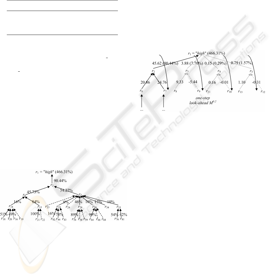
Fig. 2 shows the one step look-ahead with arrows
“stepping over” the intermediate nodes, and pointing
at the RHS variables of equation 2, 3, 4 and 5, in
the partial explanation tree. In this figure, the straight
black lines indicate the parsimonious causes that were
detected with maximal explanation.
Figure 2: Illustration of one-step look-ahead.
In the analysis phase of the procedure the function
substitution is applied to find parsimonious contribut-
ing and counteracting causes, which were missed
in the local explanation of differences by standard
multi-level explanation. Equations 2 through 5 are
substituted into the root equation and the follow-
ing new equation for explanation generation is de-
rived: M
0;2
: r
1
= (r
6
− r
7
) + (r
8
− r
9
) + (r
10
− r
11
) +
(r
12
− r
13
). This equation obtained by substitution is
added to the set of business model equations, chang-
ing the original business model. Because the substi-
tuted function is again additive, the conjunctiveness
constraint is satisfied. Notice that the specification of
the event to explain ∂r
1
remains the same, but now
equation M
0;2
is applied to explain the difference. Ta-
ble 4 summarizes the results of our extended model
of ABC-company’s relatively high results before tax-
ation. It follows that C
+
p
= {r
6
,r
7
,r
8
} and C
−
p
= {r
9
}.
We conclude that the effects of causes r
8
and r
9
are
significant at the specified fractions for parsimonious
sets.
Notice that these hidden causes were missing in
analysis with maximal explanation. For the tree of
causes this means that two new children are added to
the root node: a contributing child for r
8
and a coun-
teracting child for r
9
. As a result the top branches of
ICEIS 2007 - International Conference on Enterprise Information Systems
126
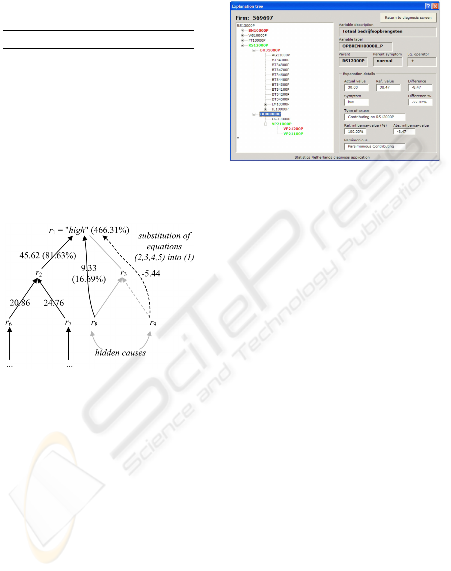
Table 4: Actual and norm values for M
0;2
: r
1
= (r
6
− r
7
) +
(r
8
− r
9
) + (r
10
− r
11
) + (r
12
− r
13
).
actual norm inf(x
i
,y) diff. %
r
1
61.75 11.30 466.31
r
6
329.50 308.64 20.86 6.76
r
7
269.09 293.84 24.76 -8.42
r
8
11.17 1.84 9.33 507.07
r
9
9.83 4.39 -5.44 123.92
r
10
0.00 0.16 0.16 -100.00
r
11
0.00 0.01 -0.01 -100.00
r
12
0.00 0.31 -0.31 -100.00
r
13
0.00 1.10 1.10 -100.00
the original tree are updated, as can be seen in Fig.
3. Notice that the variable r
3
is not part of the tree of
causes (grey line).
Figure 3: Detection of hidden causes with M
0;2
of S =
{∂r
1
= high}.
4 IMPLEMENTATION
In this section we shortly present the software imple-
mentation of the prototype diagnosis application in
MS Excel in combination with Visual Basic. This ap-
plication is initially programmed to perform the ex-
periments and analyses for the case study at Statis-
tics Netherlands. However the prototype software can
handle data and business models from multiple appli-
cation domains. Most elements of the program are
discussed in the previous parts of this paper. How-
ever the procedure diagnostic component was not dis-
cussed earlier. It contains the method for maximal
explanation as well as the multi-step look-ahead al-
gorithm. For the implementation of the procedure
we applied tree programming to generate the tree of
causes.
Figure 4: Tree viewer in diagnosis application.
The tree-viewer interface of the program is de-
picted in Fig. 4. In the viewer the whole explanatory
graph can be made visible my manipulating the tree.
In addition, the tree of causes is projected on the ex-
planatory graph by highlighting parsimonious causes
with a colour. By clicking on the cause under consid-
eration the details for the cause become visible in the
right panel of the screen.
5 SUMMARY AND CONCLUSION
In this paper, we extended the method for automated
business diagnosis in (Daniels and Feelders, 2001;
Feelders, 1993) and developed a new implementation.
The explanation model is extended in two ways: in
the symptom detection phase the probability distri-
bution of business model variables is taken into ac-
count and in the explanation generation phase hidden
causes can be made visible by function substitution.
The problem of looking for exceptional company be-
haviour in financial data sets is translated into the
problem of looking for exceptional normalized resid-
uals. Furthermore, the multi-level look-ahead algo-
rithm is proposed to enhance the explanation method-
ology so that it can deal with cancelling-out effects,
i.e. the common effect that variables cancel each
other out somewhere in the business model with the
result that their effect on a higher level in the business
model is partially or fully neutralized. The extended
model is implemented in VB. Within the software im-
plementation special attention is given to presentation
of the program output, where symptoms and causes
are presented graphically as a tree of causes. In this
manner, a manager or financial analyst can view and
access the results of the explanation process for diag-
EXPLANATION GENERATION IN BUSINESS PERFORMANCE MODELS - With a Case Study in Competition
Benchmarking
127

nosis of company performance as a compact tree.
The applicability of the method is illustrated in
a case study on interfirm/historic comparison in the
Dutch retail and wholesale trade, based on produc-
tion statistics obtained from Statistics Netherlands.
In the case study it is shown that in the presence of
cancelling-out effects the extended model with the
multi-level look-ahead procedure makes significant
causes visible that would be missed by the explana-
tion methodology of maximal explanation. In addi-
tion, the fully automated diagnostic process makes it
possible to detect and explain abnormal company be-
haviour in large data sets. We believe that this en-
hanced framework could assist analysts and improve
the decision-making process, by automatically gener-
ating explanations for exceptional values in various
data sets and business models.
REFERENCES
Courtney, J. F., Paradice, D. B., and Mohammed, N. H. A.
(1987). A knowledge-based dss for managerial prob-
lem diagnosis. Decision Sciences, 18(3):373–399.
Daniels, H. A. M. and Feelders, A. J. (2001). A general
model for automated business diagno sis. European
Journal of Operational Research, 130:623–637.
Feelders, A. J. (1993). Diagnostic reasoning and expla-
nation in financial models of the firm. PhD thesis,
Tilburg University, Department of Econo mics.
Hesslow, G. (1983). Explaining differences and weighting
causes. Theoria, 49:87–111.
Humphreys, P. W. (1989). The chances of explanation.
Princeton University Press, New Jersey.
Kosy, D. W. and Wise, B. P. (1984). Self-explanatory fi-
nancial planning models. In Proc. of AAAI-84, pages
176–181, Austin, TX.
Pounds, W. F. (1969). The process of problem finding. In-
dustrial Management Review, 11(1):1–19.
Statistics Netherlands (2006). Centraal bureau voor de
statistiek.
Verkooijen, W. J. (1993). Automated financial diagnosis: a
comparison with other diagnostic domains. J. Inf. Sci.,
19(2):125–135.
APPENDIX
Because of space limitations only the description of the
variables identified by the explanation model are described
here in detail.
Result variables:
r
6
: total operating revenues
r
7
: total operating costs
r
8
: financial revenues
r
9
: financial expenses
r
10
: additions to allowances
r
11
: deductions from allowances and provisions released
r
12
: extraordinary profits
r
13
: extraordinary losses
Revenue variables:
r
14
: total additional revenues
r
15
: total net sales
.
.
.
r
22
: net sales other activities
Cost variables:
r
23
: cost of goods sold
r
24
: total costs of labour
.
.
.
r
34
: depreciations on tangible and intangible fixed assets
Algorithm: Multi-level Look-ahead
1: y is the root node of the tree
2: for p = 0 to N − 1 do
3: determine parsimonious causes for equation(s)
M
p;p+1
4: add parsimonious causes to the tree as successor
nodes
5: if look-ahead is activated then
6: for i = 1 to N − 1 do
7: substitute jointly all equations on M
p+i;p+i+1
into equation M
p;p+i
8: add derived equation M
p;p+i+1
to M
9: determine parsimonious causes for M
p;p+i+1
10: if causes on level p + i + 1 are parsimonious
then
11: add new parsimonious causes as successor
nodes to the tree
12: remove non-parsimonious causes from the
tree
13: if a node corresponds to counteracting cause then
14: it has no successors
15: if a node corresponds to variable that cannot be ex-
plained in M then
16: it has no successors
ICEIS 2007 - International Conference on Enterprise Information Systems
128
