A NEW ALGORITHM FOR TWIG PATTERN MATCHING

Yangjun Chen

Dept. Applied Computer Science, University of Winnipeg, Canada

Keywords: XML databases, Trees, Paths, XML pattern matching, Twig joins.

Abstract: Tree pattern matching is one of the most fundamental tasks for XML query processing. Prior work has

typically decomposed the twig pattern into binary structural (parent-child and ancestor-descendent)

relationships or paths, and then stitch together these basic matches by join operations. In this paper, we

propose a new algorithm that explores both the document tree and the twig pattern in a bottom-up way and

show that the join operation can be completely avoided. The new algorithm runs in O(|T|⋅|Q|) time and

O(|Q|⋅leaf

) space, where T and Q are the document tree and the twig pattern query, respectively; and leaf

represents the number of leaf nodes in T. Our experiments show that our method is effective, scalable and

efficient in evaluating twig pattern queries.

1 INTRODUCTION

In XML, data is represented as a tree; associated

with each node of the tree is an element type from a

finite alphabet ∑. The children of a node are ordered

from left to right, and represent the content (i.e., list

of subelements) of that element.

To abstract from existing query languages for XML

(e.g. XPath, XQuery, XML-QL, and Quilt), we

express queries as twig patterns (or say, tree

patterns) where nodes are types from ∑ ∪ {*} (* is a

wildcard, matching any node type) and string values,

and edges are parent-child or ancestor-descendant

relationships. As an example, consider the query tree

shown in Fig. 1, which asks for any node of type b

(node 2) that is a child of some node of type a (node

1). In addition, the b type (node 2) is the parent of

some c type (node 4) and an ancestor of some d type

(node 5). Type b (node 3) can also be the parent of

some e type (node 7). The query corresponds to the

following XPath expression:

a[b[c and //d]]/b[c and e//d].

In this figure, there are two kinds of edges: child

edges (c-edges) for parent-child relationships, and

descendant edges (d-edges) for ancestor-descendant

relationships. A c-edge from node v to node u is

denoted by v → u in the text, and represented by a

single arc; u is called a c-child of v. A d-edge is

denoted v ⇒ u in the text, and represented by a

double arc; u is called a d-child of u.

Definition 1. An embedding of a twig pattern Q into

an XML document T is a mapping f: Q → T, from

the nodes of Q to the nodes of T, which satisfies the

following conditions:

(i) Preserve node type: For each u ∈ Q, u and f(u)

are of the same type. (or more generally, u’s

predicate is satisfied by f(u).)

(ii) Preserve c/d-child relationships: If u → v in Q,

then f(v) is a child of f(u) in T; if u ⇒ v in Q,

then f(v) is a descendant of f(u) in T.

If there exits a mapping from Q into T, we say, Q

can be imbedded into T, or say, T contains Q. In

addition, if label(T’s root) = label(Q’s root), we say

that the embedding is root-preserving.

As an example, see the document tree and the

twig pattern shown in Fig. 2(a).

There exits a mapping from Q to T as illustrated

by the dashed lines, by which each node of Q is

mapped to a different node of T. However,

according to the definition, an embedding could map

several nodes of Q (of the same type) to the same

node of T, as shown in Fig. 2(b), by which nodes q

and q

in Q are mapped onto a single node v

in T,

and q

are mapped onto a single node v

in T.

4 c d 5

2 b

d 8

1 a

6 c

b 3

e 7

Figure 1: A query tree.

Chen Y. (2007).

A NEW ALGORITHM FOR TWIG PATTERN MATCHING.

In Proceedings of the Ninth International Conference on Enterprise Information Systems - DISI, pages 44-51

DOI: 10.5220/0002356300440051

 SciTePress

For the purpose of query evaluation, either of the

mappings is recognized as a tree embedding.

In fact, almost all the existing strategies are

designed to work in this way.

In this paper, we discuss a new algorithm, which

works in a bottom-up way and shows that the join or

join-like operations can be completely avoided. The

algorithm works in O(|T|⋅|Q|) time and O(|Q|⋅leaf

)

space, where leaf

is the number of the leaf nodes of

The remainder of the paper is organized as

follows. In Section 2, we review the related work. In

Section 3, we discuss our main algorithm. Section 4

is devoted to the implementation and experiments.

Finally, a short conclusion is set forth in Section 5.

2 RELATED WORK

With the growing importance of XML in data

exchange, the tree pattern queries over XML

documents have been extensively studied recently.

Most existing techniques rely on indexing or on the

tree encoding to capture the structural relationships

among document elements.

XISS (Li and Moon, 2001) is a typical method

based on indexing, by which single

elements/attributes are indexed as the basic unit of

query and a complex path expression is decomposed

into a set of basic path expressions. Then, atom

expressions (single elements or attributes) are

recognized by direct accessing the index structure.

All other kinds of expressions need join operations

to stitch individual components together to get the

final results.

Paths are also used as the basic indexing unit as

done by DataGuide (Goldman and Widom, 1997)

and Fabric (Cooper and et al., 2001). By DataGuide,

a concise summary of path structures for a semi-

structured database is provided, but restricted to row

paths. No complex path expressions or regular

expression queries can be handled. Fabric works

better in the sense that the so-called refined paths are

supported. Such queries may contain branches, wild-

cards (*) and ancestor-descendent operators (//).

However, any query not in the set of refined paths

has to resort to join operations. Another two

strategies based on the path indexing are APEX

(Chung and et al., 2002) and F

B (Kaushik and et

al., 2002). APEX is an adaptive path index and uses

data mining technique to summarize paths that

frequently appear in the query workload. It has to be

updated as the query workload changes. In stead of

maintaining all paths starting from the root, it keeps

every path segment of length 2. Obviously, to get the

final results, the join operations have to be

conducted. F

B (Kaushik and et al., 2002) shares the

flavour of Fabric (Cooper and et al., 2001). It is

based on the so-called forward and backward index

(F&G index (Abiteboul and et al., 1999)), which

covers all the branching paths. It works well for pre-

defined query types. In normal cases, however, such

a set of F&B indexes tends to be large and therefore

the performance suffers. The method discussed in

(Wang and et al., 2003) can be considered as a quite

different method, by which a document is stored as a

sequence: (a

, p

), ..., (a

, p

), ..., (a

, p

), where each

is an element or a word in the document, and p

path from the root to it. Using this method, the join

operations are replaced by searching a trie structure

(called suffix tree in (Wang and et al., 2003)). The

drawback of this method is that a relatively large

index structure has to be created. Another problem

of this method is that a document tree that does not

contain a query pattern may be designated as one of

the answers due the ambiguity caused by identical

sibling nodes. This problem is removed by the so-

called forward prefix checking discussed in (Wang

and Meng, 2005). Doing so, however, the theoretical

time complexity is dramatically increased.

All the above methods need to decompose a twig

pattern into a set of binary relationships between

pairs of nodes, such as parent-child and ancestor-

descendant relations, or into a set of paths. The sizes

of intermediate relations tend to be very large, even

when the input and final result sizes are much more

manageable. As an important improvement,

TwigStack was proposed by Bruno et al. (Bruno and

et al., 2002), which compress the intermediate

results by the stack encoding, which represents in

linear space a potentially exponential number of

answers. However, TwigStack achieves optimality

c v

b v

a v

c c v

c q

b q

(a)

c v

b v

a v

c c v

c q

b q

(b)

Figure 2: Illustration for tree embedding.

A NEW ALGORITHM FOR TWIG PATTERN MATCHING

only for the queries that contain only d-edges. In the

case that a query contains both c-edges and d-edges,

some useless path matchings have to be performed.

In addition, in the worst case, TwigStack needs

O(|D|

Q|) time for doing the merge joins as shown by

Chen et al. (see page 287 in (Chen and et al., 2006)),

where D is a largest data stream associated with a

node q in Q, which contains all the document nodes

that match q. Since then, several methods that

improve TwigStack in some way have been reported.

For instance, iTwigJoin (Chen and et al., 2005)

exploits different data partition possibilities while

TJFast (Lu and et al., 2005) accesses only leaf nodes

of document trees by using Dewey IDs. But both of

them still need to do some useless matchings as

shown by the theoretical analysis made in (Choi and

et al., 2003). Twig

Stack (Chen and et al., 2006) is

the most recent method that improves TwigStack. By

this method, the stack encoding is replaced with the

hierarchical stack encoding, by which each stack

associated with a query node contains an ordered

sequence of stack trees. In this way, the path joins

are replaced by the so called result enumeration. In

(Chen and et al., 2006), it is claimed that Twig

Stack

needs only O(|D|⋅|Q| + |subTwigResults|) time. But a

careful analysis shows that the time complexity of

the method is actually bounded by O(|D|⋅|Q|

|subTwigResults|). It is because each time a node is

inserted into a stack associated with a node in Q, not

only the position of this node in a tree within that

stack has to be determined, but a link from this node

to a node in some other stack has to be constructed,

which requires to search all the other stacks. The

number of these stacks is |Q| (see Fig. 4 in (Chen

and et al., 2006) to know the working process.)

The method discussed in (Aghili and et al., 2006)

incorporates a binary labeling as a pre-processing

filtration step to reduce the search space. This

method is effective only for the case that selective

key words at leaf nodes are specified in queries.

Finally, we point out that the bottom-up tree

matching was first proposed in (Hoffmann and

O’Donnell, 1982). But it concerns a very strict tree

matching, by which the matching of an edge to a

path is not allowed. In (Gottlob and et al., 2005), an

XPath is transformed into a parse tree and then

evaluated bottom-up or top-down. Both the bottom-

up and top-down strategies need O(|T|

⋅|Q|

) time

and O(|T|

⋅|Q|

) space. In (Miklau and Suciu, 2004),

an algorithm for tree homomorphism is discussed,

which is able to check whether a tree contains

another and returns only a boolean answer. But our

algorithms show all the subtrees than match a given

twig pattern query.

In comparison with the above methods, our

methods have the following advantages:

- Our first algorithm needs less time than

Twig

Stack. Concretely, our algorithm runs in

O(|D|⋅|Q|) time.

- Neither matching paths nor tree stacks are

generated. Therefore, the costly path joins (Aghili

and et al., 2006), as well as the result

enumeration, a join-like operation (Chen and et

al., 2006), are not needed.

- The runtime memory usage is minimum. During

the process, our algorithm transforms

(dynamically) the data streams to a tree structure

T with all the matching patterns recognized. To

represent the results, each node v in T is

associated with a set of nodes in Q (denoted as

M(v)) such that for each q ∈ M(v) the subtree

rooted at q can be embedded in the subtree rooted

at v. If M(v) contains the root of Q, it indicates an

answer and v will be stored in a global variable (or

report the subtree rooted at v as an answer). Later

on, M(v) will be removed once M(v’s parent) is

established since M(v) will not be accessed any

more.

3 ALGORITHM

In this section, we discuss our algorithm according

to Definition 1. The main idea of this algorithm is to

search both T and Q bottom-up and checking the

subtree embedding by generating dynamic data

structures. In the process, a tree labeling technique is

used to facilitate the recognition of nodes’

relationships. Therefore, in the following, we will

first show the tree labeling in 3.1. Then, in 3.2, we

discuss the main algorithm. In 3.3, we prove the

correctness of the algorithm and analyze its

computational complexities.

3.1 Tree Labeling

Before we give our main algorithm, we first restate

how to label a tree to speed up the recognition of the

relationships among the nodes of trees.

Consider a tree T. By traversing T in preorder,

each node v will obtain a number (it can an integer

or a real number) pre(v) to record the order in which

the nodes of the tree are visited. In a similar way, by

traversing T in postorder, each node v will get

another number post(v). These two numbers can be

used to characterize the ancestor-descendant

relationships as follows.

ICEIS 2007 - International Conference on Enterprise Information Systems

Proposition 1. Let v and v’ be two nodes of a tree T.

Then, v’ is a descendant of v iff pre(v’) > pre(v) and

post(v’) < post(v).

Proof. See Exercise 2.3.2-20 in [34].

If v’ is a descendant of v, then we know that

pre(v’) > pre(v) according to the preorder search.

Now we assume that post(v’) > post(v). Then,

according to the postorder search, either v’ is in

some subtree on the right side of v, or v is in the

subtree rooted at v’, which contradicts the fact that

v’ is a descendant of v. Therefore, post(v’) must be

less than post(v). The following example helps for

illustration.

Example 1. See the pairs associated with the nodes

of the tree shown in Fig. 3. The first element of each

pair is the preorder number of the corresponding

node and the second is its postorder number. With

such labels, the ancestor-descendant relationships

can be easily checked.

For instance, by checking the label associated with

against the label for v

, we see that v

is an

ancestor of v

in terms of Proposition 1. Note that

’s label is (2, 6) and v

’s label is (6, 3), and we

have 2 < 6 and 6 > 3. We also see that since the pairs

associated with v

and v

do not satisfy the condition

given in Proposition 1, v

must not be an ancestor of

and vice versa.

Definition 1. (label pair subsumption) Let (p, q) and

(p’, q’) be two pairs associated with nodes u and v.

We say that (p, q) is subsumed by (p’, q’), denoted

(p, q) (p’, q’), if p > p’ and q < q’. Then, u is a

descendant of v if (p, q) is subsumed by (p’, q’).

In the following, we also use T[v] to represent a

subtree rooted at v in T.

3.2 Algorithm for Twig Pattern

Matching

Now we discuss our algorithm for twig pattern

matching. During the process, both T and Q are

searched bottom-up. That is, the nodes in T and Q

will be accessed along their postorder numbers.

Therefore, for convenience, we refer to the nodes in

T and Q by their postorder numbers, instead of their

node names.

In each step, we will check a node j in T against

all the nodes i in Q.

In order to know whether Q[i] can be embedded

into T[i], we will check whether the following two

conditions are satisfied.

1. label(j) = label(i).

2. Let i

, ..., i

be the child nodes of i. For each i

(a =

1, ..., k), if (i, i

) is a c-edge, there exists a child

node j

of j such that T[j

] contains Q[i

]; if (i, i

)

is a d-edge, there is a descendent j’ of j such that

T[j’] contains Q[i

To facilitate this process, we will associate each j

in T with a set of nodes in Q: {i

, ..., i

} such that for

each i

∈ {i

, ..., i

} Q[i

] can be root-preservingly

embedded into T[j]. This set is denoted as M(j). In

addition, each i in Q is associated with a value β(i),

defined as below.

i) Initially, β(i) is set to φ.

ii) During the computation process, β(i) is

dynamically changed. Concretely, each time we

meet a node j in T, if i appears in M(j

) for some

child node j

of j, then β(i) is changed to j.

In terms of above discussion, we give the

following algorithm.

Algorithm Twig-pattern-matching(T, Q)

Input: tree T (with nodes 0, 1, ..., |T|) and tree Q (with

nodes 1, ..., |Q|)

Output: a set of nodes j in T such that T[j] contains Q.

begin

1. for j := 1, ..., |T| do

2. {let j

, ..., j

be the children of j;

3. for l := 1, ..., k do

4. {for each i’ ∈ M( j

) do β(i’) ← j;

5. remove Μ( j

);}

5. for i := 1, ..., |Q| do

6. if label(i) = label(j) then

7. {let i

, ..., i

be the children of i;

8. if for each i

(l = 1, ..., g) we have

9. (i, i

) is a c-edge and β(i

) = j, or

10. (i, i

) is a d-edge and β(i

) is subsumed by j;

11. then {insert i into M(j);

12. if i is the root of Q, then report the subtree

rooted at j as an answer;}

13. }

end

In the above algorithm, each time we meet an j in

T, we will establish the new β values for all those

nodes of Q, which appear in

), ...,

), where

, ..., j

represent the child nodes of j (see lines 1 -

4). Then, all

)’s (l = 1, ..., k) are removed. In a

next step, we will check j against all the nodes i in Q

(see lines 5 - 13). If label(i) = label(j), we will check

β(i

), ..., β(i

), where i

, ..., i

are the child nodes of i.

If (i, i

) (l ∈ {1, ..., g}) is a c-edge, we need to check

A v

B v

C v

(1, 8)

(2, 6)

(3, 1)

(4, 5)

(5, 2)

(8, 7)

C v

(6, 3)

(7, 4)

Figure 3: Illustration for tree encoding.

A NEW ALGORITHM FOR TWIG PATTERN MATCHING

whether β(i

) = j (see line 9). If (i, i

) (l ∈ {1, ..., g})

is a d-edge, we simply check whether β(i

) is

subsumed by j (see line 10). If all the child nodes of

i survive the above checking, we get a root-

preserving embedding of the subtree rooted at i into

the subtree rooted at j. In this case, we will insert j

into M(j) (see line 11) and report j as one of the

answers if i is the root of Q (see line 12).

Example 2. Consider the document tree T and the

twig pattern query Q shown in Fig. 2(a) once again.

When applying the above algorithm to T and Q, we

will find that Q can be root-preservingly embedded

into T. Fig. 4 shows the whole computation process.

In the first four steps, we check respectively v

, v

, and v

against Q, generating a data structure as

shown in Fig. 4(a), in which M(v

) = M(v

)

= {q

, q

} and M(v

) = { }. In a next step, we meet v

and generate a data structure as shown in Fig. 4(b).

In more detail, in this step, we first set β(q

) =

and

β(q

) =

, and then try to find any subtree in Q,

which can be embedded into T[v

]. Since label(v

) =

label(q

) = B and both β(q

) and β(q

) are equal to

, it shows that T[v

] contains Q[q

]. So M(v

)

contains q

. In addition, since q

is a leaf node (no

children) and label(v

) = label(q

), M(v

) also

contains q

. In the sixth step, we will meet v

and the

data structure generated is shown in Fig. 4(c). Here,

we should remark that not only β(q

) and β(q

) are

set to v

, but β(q

) and β(q

) are also changed to v

It is because in this step we have M(v

) = {q

, q

}

and v

is a child node of v

. Therefore, we have

M(v

) = {q

, q

}. In the seventh step, we meet v

and

generate a data structure as shown in Fig. 4(d).

Although we have label(v

) = label(q

), we cannot

insert q

into M(v

) since in this step both β(q

) and

β(q

) are equal to v

, not to v

. So M(v

) contains

only q

. In the final step, we meet v

. The

corresponding data structure is shown in Fig. 4(e).

Since M(v

) contains q

, the root of Q, we know that

Q can be embedded into T.

4 CORRECTNESS AND

COMPUTATIONAL

COMPLEXITIES

In this subsection, we show the correctness of the

algorithm given in 3.2 and analyze its computational

complexity.

- Correctness

The correctness of the algorithm consists in a

very important property of postorder numbering

described in the following lemma.

Lemma 1. Let v

, v

, and v

be three nodes in a tree

with post(v

) < post(v

). If v

is a

descendent of v

. Then, v

must also be a descendent

of v

Proof. We consider two cases: i) v

is to the right of

, and ii) v

is an ancestor of v

. In case (i), we have

post(v

) < post(v

). So we have pre(v

) < pre(v

) <

pre(v

). This shows that v

is a descendent of v

. In

case (ii), v

, v

, and v

are on the same path. Since

post(v

) < post(v

), v

must be a descendent of v

We illustrate Lemma 1 by Fig. 5, which is helpful

for understanding the proof of Proposition 2 given

below.

Proposition 2. Let Q be a twig pattern containing

only d-edges. Let v be a node in the document tree T.

Let q

be a node in Q. Then, q

appears in M(v) if and

only if T[v] contains Q[q].

Proof. If-part. A query node q is inserted into M(v)

by executing lines 6 - 11 in Algorithm Twig-pattern-

matching( ). Obviously, for any q

inserted into M(v)

we must have T[v] containing Q[q].

Only-if-part. Assume that there exists a q

in Q such

that T[v] contains Q[q] but q does not appear in

M(v). Then, there must be a child node q

of q

such

that (i) β(q

) =

, or (ii) β(q

) is not subsumed by v.

Obviously, case (i) is not possible since T[v]

Figure: 4: A sample trace.

•

• B {q

, q

}

• B

• C

)=v

}

• B

)=v

•

• C

}

• B

(d)

(a)

• C

, q

}

• C

, q

}

• C

, q

}

• D

• C

, q

}

{}

• B {q

, q

}

)=v

•

(

)

(c)

• B

)=v

•

• C

• B

• B { q

}

(e)

• v

Figure 5: A matching subtree with M’s.

is to the right of v

; or

appears as an ancestor of v

, but

as a descendant of v

• v

ICEIS 2007 - International Conference on Enterprise Information Systems

contains Q[q] and q

must be contained in a subtree

rooted at a node v’ which is a descendent of v. So

β(q

) will be changed to a value not equal to

. Now

we show that case (ii) is not possible, either. First,

we note that during the whole process, β(q

) may be

changed several times since it may appear in more

than one M’s. Assume that there exist a sequence of

nodes v

, ..., v

for some k ≥ 1 with post(v

) <

post(v

) <... < post(v

) such that q

appears in M(v

..., M(v

). Without loss of generality, assume that v’

= v

for some i ∈ {1, ..., k} and there exists an j such

that post(v

) < post(v) < post(v

j+1

). Then, at the time

point when we check q, the actual value of β(q

) is

the postorder number for v

’s parent, which is equal

to v or whose postorder number is smaller than

post(v). If it is equal to v, then β(q

) is subsumed by

v, contradicting (ii). If post(β(q

) is smaller than

post(v). Thus, we have

post(v’) < post(β(q

) < post(v).

In terms of Lemma 1, the value of β(q

) is a

descendent of v and therefore subsumed by v. The

above explanation shows that case (ii) is impossible.

This completes the proof of the proposition.

Lemma 1 helps to clarify the only-if part of the

above proof. In fact, it reveals an important property

of the tree encoding, which enables us to save both

space and time. That is, it is not necessary for us to

keep all the values of β(q

), but only one to check the

ancestor-descendent relationship. Due to this

property, the path join (Bruno and et al., 2002), as

well as the result enumeration (Chen and et al.,

2006), can be completely avoided.

Concerning the correctness of the general case

that Q contains both c-edges and d-edges, we have

to answer a question: whether any c-edge in Q is

correctly checked.

To answer this question, we note that any c-edge in

Q cannot be matched to any path with length larger

than 1in T. That is, it can be matched only to a c-

edge in T. It is exactly what is done by the

algorithm. See Fig. 6 for illustration.

Each time we meet a node v, we will set β values for

all those q

’s that appear in an M associated with

some child node of v (see lines 3 - 4). Then, in lines

9 - 10, when we check whether q can be inserted

into M(v), any outgoing c-edge of q is correctly

checked. As shown in Fig. 6, after the value of β(q

)

is set to be v, q is checked and the value of β(q

)

indicates that v’ is a child of v. Since (v, v’) is also a

c-edge, it matches (q, q

). Although the value of

β(q

) is changed from v

to v during the process, it

does not impact the correctness of c-edge checkings

which use only the newly set β values that are

always the parent of the corresponding nodes.

In conjunction with Proposition 2, the above

analysis shows the correctness of the algorithm. We

have the following proposition.

Proposition 3. Let Q be a twig pattern containing

only both c-edges and d-edges. Let v be a node in T.

Let q

be a node in Q. Then, q

appears in M(v) if and

only if T[v] contains Q[q].

Proof. See the above discussion.

- Computational complexities

The time complexity of the algorithm can be

divided into two parts:

1. The first part is the time spent on generating β

values (see lines 2 - 5). For each node j in T, we

will access M(j

) for each child node j

of j.

Therefore, this part of cost is bounded by

∑

⋅

|)(|

jMd ) ≤ Ο(

∑

⋅

Qd ) = O(|T|⋅|Q|),

where d

is the outdegree of j.

2. The second part is the time used for constructing

M(j)’s. For each node j in T, we need O(

∑

c )

time to do the task, where c

is the outdegree of i in

Q, which matches j. So this part of cost is bounded

∑

c ) ≤ O(

∑

Q ) = O(|T|⋅|Q|).

The space overhead of the algorithm is easy to

analyze. During the processing, each j in T will be

associated with a M(j). But M(j) will be removed

later once j’s parent is encountered and for each i

∈ M(j) its β value is changed. Therefore, the total

space is bounded by

O(leaf

⋅|Q| + |T| + |Q|),

where leaf

represents the number of the leaf nodes

of T. It is because at any time point for any two

nodes on the same path in T only one is associated

with a M.

5 EXPERIMENTS

We conducted our experiments on a DELL desktop

PC equipped with Pentium III 864Mhz processor,

512MB RAM and 20GB hard disk. We use Oracle-

(v’) = {…, q

, …}

) has been once set to be v

(v’) = {…, q

, …}

) is changed to v when v is

recognized to be the parent of v’.

Figure 6: Illustration for c-edge checking.

a • v

a • q

c • v

b • v’ b • q

c • q

b • v

’

A NEW ALGORITHM FOR TWIG PATTERN MATCHING

9i Enterprise Edition as the working platform and

implement the algorithms in Oracle PL/SQL

language. We set the size of the buffer cache of

Oracle-9i to be 8 MBytes and the B+-tree built in the

system is used as the index.

- Tested methods

In the experiments, we have tested three methods:

TwigStack (TS for short) [4],

Twig

Stack (T

S for short) [10],

Twig-pattern-matching (discussed in this paper;

TPM for short),

and compare their execution times.

- Data

The data set used for this test is DBLP data set [24]

and a synthetic XMARK data set. The quantitative

characteristics of the sets are described below.

- DBLP. It is a computer science bibliography

database. In this data set, each author is

represented by a name, a homepage, and a list of

papers. In turn, each paper contains a title, the

conference or the journal title where it was

published, and a list of coauthors. In the version

we downloaded, there are 3,332,130 elements and

404,276 attributes, totaling 127 MBytes of data.

Each record in DBLP corresponds to a publication

which is a simple tree structure of maximum depth

6. The average length of a structure-encoded

sequence derived through the reference mechanism

in a tree is around 31. The B+-tree established on

individual publications is about 2 MBytes of data.

- XMARK. It is a popular database in benchmarking

XML index methods. It is a very large and

complicated tree structure, containing some

substructures such as regions, items (objects for

sale), people, open-auction, closed-auction, etc. In

our experiment, we generate an XMARK set by

using xmlgen with scaling factor 1.0. It contains

about 108 MBytes of data. The B+-tree established

on individual sales is about 1.3 MBytes of data.

- Queries

As we know, XML queries may have different

patterns and may or not be with parameters being

specified. To study the performance impact of these

two characteristics, we have tested 10 queries

against DBLP database, which are divided into two

groups. In the first group all the 5 queries are with a

constant while in the second group (another 5

queries) no parameter is specified. Over XMARK

database, we have also tested 10 queries, divided

into 2 groups with each containing 5 queries. In the

first group, each query contains a constant. In the

second group, for each query no constant is

specified. All the queries are shown in Table 1 -

Table 4.

Queries over DBLP:

Table 1: Group I.

query

Xpath expression

Q1 //inproceedings/[author]//year [text() = ‘1999’]

Q2 //inproceedings/[author and /title]//year [text() = ‘1999’]

Q3 //inproceedings/[author and /title and //pages]//year [text() = ‘1999’]

Q4 //inproceedings/[author and /title and //pages and //url]//year [text() =

Q5 //articles/[author and /title and //volume and //pages and //url]//year

[text() = ‘1999’]

Table 2: Group II.

query

Xpath expression

Q6 //inproceedings/[author]//year

Q7 //inproceedings/[author and /title]//year

Q8 //inproceedings/[author and /title and //pages]//year

Q9 //inproceedings/[author and /title and //pages and //url]//year

Q10 //articles/[author and /title and //volume and //pages and //url]//year

Queries over XMARK:

Table 3: Group III.

query

Xpath expression

Q11 /site//open_auction[seller/person]//date [text() = ‘10/23/1999’]

Q12 /site//open_auction[//seller/person and //bidder]//date [text() =

Q13 /site//open_auction[//seller/person and //bidder/increase]//date [text() =

‘10/23/1999’]

Q14 /site//open_auction[//seller/person and //bidder/increase and

//initial]//date [text() = ‘10/23/1999’]

Q15 /site//open_auction[//seller/person and //bidder/increase and //initial and

//description]//date [text() = ‘10/23/1999’]

Table 4: Group IV.

query

Xpath expression

Q16 /site//open_auction[seller/person]//date

Q17 /site//open_auction[//seller/person and //bidder]//date

Q18 /site//open_auction[//seller/person and //bidder/increase]//date

Q19 /site//open_auction[//seller/person and //bidder/increase and

//i i i l //d

Q20 /site//open_auction[//seller/person and //bidder/increase and //initial and

//description]//date

- Test results

Now we demonstrate the execution times of all

the four strategies when they are applied to the

above queries.

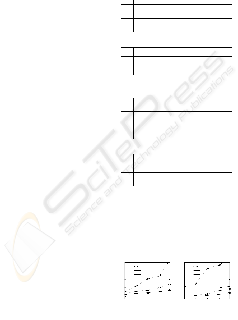
In Fig. 7(a), we show the test results of the first

group. From these we can see that our first algorithm

outperforms all the other strategies. It is because this

algorithm works only in one scan of the data streams

and neither the path join nor the result enumeration

is involved. TwigStack has the worst performance

since some path joins have to be performed.

Q1 Q2 Q3 Q 4 Q5

Exec uti o n Time (s ec. )

TPM

Q 6 Q7 Q 8 Q9 Q10

Execution Time (sec.)

TP M

(b)

(a)

Figure 7: Results of Group I and Group.

ICEIS 2007 - International Conference on Enterprise Information Systems

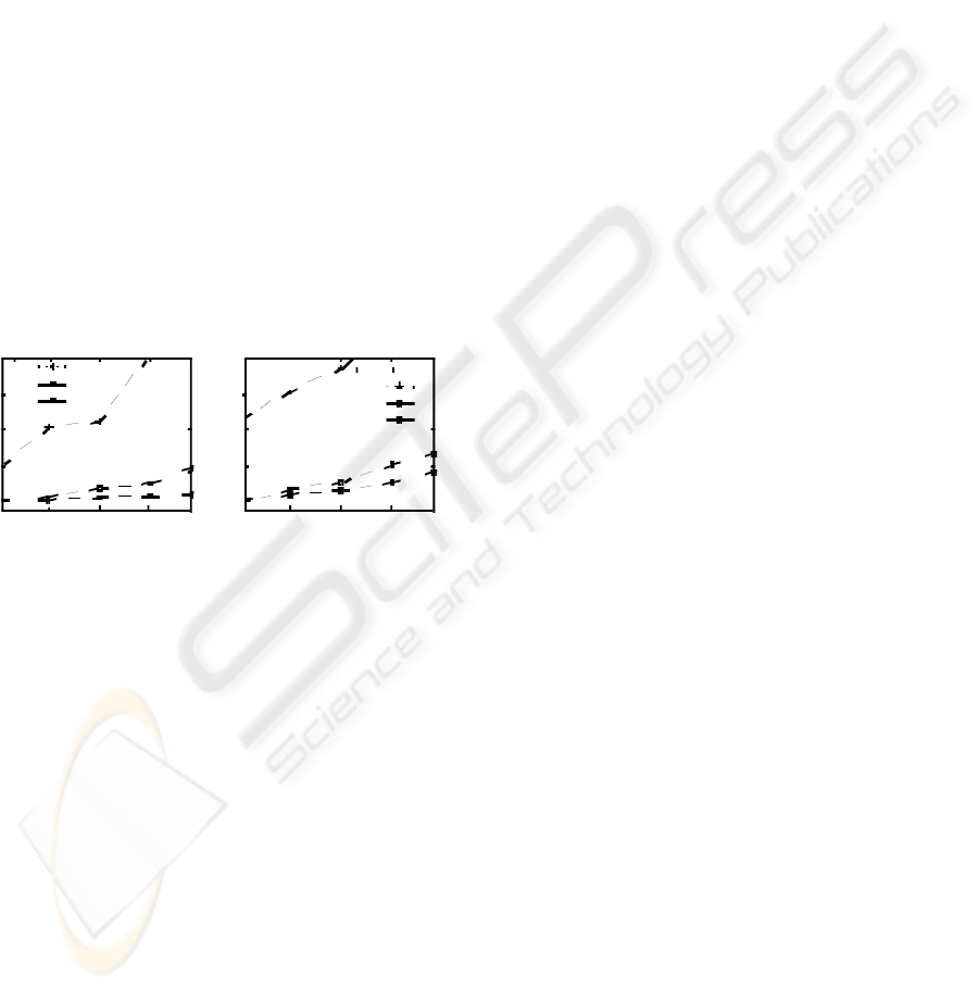
Fig. 7(b) shows the test results of the second

group. The execution time of all the strategies are

much worse than Group 1 since the queries are all of

quite low selectivity and thus almost all the data set

has to be downloaded into main memory. In this

case, I/O dominates the cost. Again, our first

algorithm has the best performance. Especially,

when the size of queries becomes larger, this

algorithm is 3 - 4 times better than Twig

Stack. First,

the time for constructing a matching tree is much

less than that for constructing the hierarchical stacks.

Secondly, the space used by our first algorithm is

much smaller than Twig

Stack. It is because our

algorithm removes useless data structures earlier

than Earlier Result enumeration utilized by

Twig

Stack. TwigStack shows an exponential-time

behavior since for each path in a query a great many

matching paths will be produced and the cost of join

operations increases exponentially.

In Fig. 8, the test results over the XMARK

database are demonstrated. From these, we can see

that our first algorithm still has the best performance

for this data set.

Q11 Q12 Q13 Q14 Q 15

Exec ut i o n T ime ( s ec. )

Q16 Q17 Q18 Q19 Q20

Execution Time (sec.)

TPM

6 CONCLUSIONS

In this paper, a new algorithm is proposed to

evaluate twig pattern queries in XML document

databases. The algorithm works in a bottom-up way,

by which an important property of the postorder

numbering is used to avoid join or join-like

operations. The time complexity and the space

complexity of the algorithm are bounded by

O(|T|

⋅|Q|) and O(|Q|⋅leaf

), respectively, where T is

the document tree and Q the twig pattern query, and

leaf

represents the number of leaf nodes in T.

Experiments have been done to compare our method

with some existing strategies, which demonstrates

that our method is highly promising in evaluating

twig pattern queries.

REFERENCES

S. Abiteboul, P. Buneman, and D. Suciu (1999) Data on

the web: from relations to semistructured data and

XML

, Morgan Kaufmann Publisher, Los Altos, CA

94022, USA, 1999.

A. Aghili, H. Li, D. Agrawal (2006). and A.E. Abbadi,

TWIX: Twig structure and content matching of

selective queries using binary labeling, in:

INFOSCALE, 2006.

N. Bruno, N. Koudas, and D. Srivastava (2002) Holistic

Twig Hoins: Optimal XML Pattern Matching, in Proc.

SIGMOD Int. Conf. on Management of Data

Madison, Wisconsin, June 2002, pp. 310-321.

C. Chung, J. Min, and K. Shim (2002). APEX: An

adaptive path index for XML data,

ACM SIGMOD,

June 2002.

S. Chen et al. (2006). Twig

Stack: Bottom-up Processing

of Generalized-Tree-Pattern Queries over XML Docu-

ments, in

Proc. VLDB, Seoul, Korea, Sept. 2006, pp.

283-323.

B.F. Cooper, N. Sample (2001). M. Franklin, A.B.

Hialtason, and M. Shadmon, A fast index for

semistructured data, in:

Proc. VLDB, Sept. 2001, pp.

341-350.

R. Goldman and J. Widom (1997). DataGuide: Enable

query formulation and optimization in semistructured

databases, in: Proc. VLDB, Aug. 1997, pp. 436-445.

G. Gottlob, C. Koch, and R. Pichler (2005). Efficient

Algorithms for Processing XPath Queries, ACM

Transaction on Database Systems

, Vol. 30, No. 2,

June 2005, pp. 444-491.

C.M. Hoffmann and M.J. O’Donnell (1982). Pattern

matching in trees,

J. ACM, 29(1):68-95, 1982.

Q. Li and B. Moon (2001) Indexing and Querying XML

data for regular path expressions, in: Proc. VLDB,

Sept. 2001, pp. 361-370.

J. Lu, T.W. Ling, C.Y. Chan, and T. Chan (2005). From

Region Encoding to Extended Dewey: on Efficient

Processing of XML Twig Pattern Matching, in:

Proc.

VLDB

, pp. 193 - 204, 2005.

G. Miklau and D. Suciu (2004) Containment and

Equivalence of a Fragment of XPath, J. ACM, 51(1):2-

45, 2004.

H. Wang, S. Park, W. Fan, and P.S. Yu (2003) ViST: A

Dynamic Index Method for Querying XML Data by

Tree Structures, SIGMOD Int. Conf. on Management

of Data

, San Diego, CA., June 2003.

H. Wang and X. Meng (2005), On the Sequencing of Tree

Structures for XML Indexing, in

Proc. Conf. Data En-

gineering

, Tokyo, Japan, April, 2005, pp. 372-385.

R. Kaushik, P. Bohannon, J. Naughton, and H. Korth

(2002) Covering indexes for branching path queries,

in:

ACM SIGMOD, June 2002.

(b)

(a)

Figure 8: Results of Group III and Group IV.

A NEW ALGORITHM FOR TWIG PATTERN MATCHING