
DISTRIBUTED APPROACH OF CONTINUOUS QUERIES WITH
KNN JOIN PROCESSING IN SPATIAL DATA WAREHOUSE
Marcin Gorawski and Wojciech Gębczyk
Silesian Technical University, Institute of Computer Science, Akademicka 16, 44-100 Gliwice, Poland
Keywords: kNN join processing, distributed spatial data warehouse, continuous query, mobile query, mobile object.
Abstract: The paper describes realization of distributed approach to continuous queries with kNN join processing in a
spatial telemetric data warehouse. Due to dispersion of the developed system, new structural members were
distinguished - the mobile object simulator, the kNN join processing service and the query manager.
Distributed tasks communicate using JAVA RMI. The kNN queries (k Nearest Neighbour) joins every point
from one dataset with its k nearest neighbours in the other dataset. In our approach we use the Gorder
method, which is a block nested loop join algorithm that exploits sorting, join scheduling and distance
computation filtering to reduce CPU and I/O usage.
1 INTRODUCTION
With expansion of location-aware technologies such
as the GPS (Global Positioning System) and
growing popularity and accessibility of the mobile
communication, location-aware data management
becomes a significant problem in the mobile
computing systems. Mobile devices become much
more available with concurrent growth of their
computational capabilities. It is expected that future
mobile applications will require scalable architecture
that will be able to process a very large and quickly
growing number of mobile objects and to evaluate
compound queries over their locations (Yiu,
Papdias, Mamoulis, Tao, 2006).
The paper describes realization of distributed
approach to the Spatial Location and Telemetric
Data Warehouse (SDW(l/t)), which bases on the
Spatial Telemetric Data Warehouse (STDW))
STDW consist of telemetric data containing
information about water, gas, heat or electricity
consumption (Gorawski, Wróbel, 2005). DSDW(l/t)
(Distributed Spatial Location and Telemetric Data
Warehouse) is supplied by datasets from Integrated
Meter Reading (IMR) data system and by mobile
objects locations.
Integrated Meter Reading data system enables
communication between medium meters and
telemetric database system. Using GPRS or SMS
technology, measurements from meters located on a
wide geographical area are transferred into database,
where they are processed and stored for further
analysis.
The SDW(l/t) supports tactical decisions making
process concerning medium productivity on the base
of short-termed consumption predictions.
Predictions are supported in the analysis of data
assembled in a data warehouse during the ETL
process, evaluated for datasets from the telemetric
database server.
2 DESIGNED APPROACH
First figure illustrates designed approach’s
architecture. We can observe multiple, concurrently
operating mobile objects (query points), the Gorder
(Chenyi, Hongjun, Beng Chin, Jing 2004) service is
responsible for processing simultaneous continuous
queries over k nearest neighbors, RMI’s SDWServer
and the central part of designed data system -
SDW(l/t), which is also described as a query
manager. Communication between SDW(l/t) and
query processing service is maintained with Java’s
Remote Method Invocation (RMI) solutions.
Principal notion of the described approach is to
distribute previously designed system over many
independent nodes. Asa result we expect faster and
more efficient processing of similarity join method
Gorder. In the previous approach all components of
the system shown in figure 1 were linked together on
a single computer station. All active processes used
131
Gorawski M. and GÄ
´
Zbczyk W. (2007).
DISTRIBUTED APPROACH OF CONTINUOUS QUERIES WITH KNN JOIN PROCESSING IN SPATIAL DATA WAREHOUSE.
In Proceedings of the Ninth International Conference on Enterprise Information Systems - DISI, pages 131-136
DOI: 10.5220/0002368501310136
Copyright
c
SciTePress

the same CPU. Because of high CPU usage and long
evaluation time we decided to distribute the SDW
(l/t) into independent services, linked together with
Java RMI technology. The most efficient solution
assumes running the Gorder service on a separate
computer because it is the most CPU consuming
element. Other components may be executed on
other computers or on the same computer due to
their insignificant CPU consumption.
Designed system works as follows. First we have
to upload a road map and defined meters into
database on Oracle Server, using SDW(l/t). Then we
start the SDWServer, the Gorder service and as
many mobile objects as we want to evaluate. Every
new mobile object is registered in the database. In
SDW(l/t) we define new queries for active mobile
objects. Queries are also registered in database. The
Gorder service periodically verifies if any queries
are defined. Every query is processed during each
cycle of the Gorder process. The results are sent to
SDW(l/t), where they are stored for further analysis.
SDWServer secures steady RMI connection between
running processes.
Figure 1: DSDW(l/t).
3 MOBILE OBJECT’S
SIMULATOR
For designed approach’s evaluation we developed a
mobile object simulator that corresponds to any
moving object like car, man or airplane. Being in
constant movement, mobile objects are perfect to act
as a query points. Continuous changes in their
locations forces data system to continuously process
queries to maintain up-to-date information about
object’s k nearest neighbours. While designing the
mobile object mechanism we made a few
assumptions. On the one hand, mobile objects are
not allowed to interfere in system’s behaviour, but
on the other hand, they provide everything that is
necessary to conduct system’s overall experiments.
They also prepare system for realistic, natural
conditions.
Mobile object’s simulator is a single process that
represents a moving object. It consantly changes its
actual location and destination. We assume that a
moving object has the ability to send updates on its
location to the Oracle server, which is the core of
DSDW (l/t). It is justifiable assumption because the
GPS devices are getting cheaper every day.
In real terms, the location-aware monitoring
systems are not aware of mobile object’s problem of
choosing the right direction, because it is not the
system that decides where specific object is aiming
to. System only receives information about current
object’s location and makes proper decisions on the
way of processing it. Since our project is not a real
life system, but only a simulation, which goal is to
evaluate new solutions, we do not have access to the
central system containing information about the
mobile objects positions. Therefore, we had to
develop an algorithm that will decide on mobile
object’s movement in order to make SDW(l/t) more
realistic.
4 GORDER QUERY SERVICE
k Nearest Neighbor (kNN) join combines each point
of one dataset R with its k nearest neighbors in the
other dataset S. Gorder is a block nested loop join
algorithm which achieves its efficiency due to data
sorting, join scheduling and distance computation
reduction. Firstly it sorts input datasets into order
called G-order (an order based on a grid). As a
result, the datasets are ready to be partitioned into
blocks that are proper for efficient scheduling for
join processing. Secondly, scheduled block nested
loop join algorithm is applied to find k nearest
neighbors for each block of R data points within data
blocks of S dataset.
Gorder achieves its efficiency due to inheritance
of strength of the block nested loop join in being
able to reduce random reads and due to a pruning
strategy, which reduces unpromising data blocks
using properties of G-ordered data. Furthermore,
Gorder utilizes two-tier partitioning strategy to
optimize CPU and I/O time and reduces distance
computation cost by pruning away redundant
computations.
jdbc
jdbc
jdbc
jdbc
jdbc
SDWServer
RMI
ORACLE
Server
Mobile
object
Mobile
object
Mobile
object
Mobile
object
SDW(l/t)
Gorder
jdbc RMI
ICEIS 2007 - International Conference on Enterprise Information Systems
132

4.1 G-ordering
The Gorder’s authors designed an ordering based on
a grid called G-ordering to group neighboring data
points together, so that in the scheduled block nested
loop join phase they can identify the partition of a
block of G-ordered data and schedule it for join.
Firstly, Gorder conducts the PCA transformation
(Principal Component Analysis) on input datasets.
Secondly, it applies a grid on a data space and
partitions it into l
d
square cells, where l is the
number of segments per dimension.
Definition 1. (kNN join) (Chenyi, Hongjun, Beng
Chin, Jing, 2004) Given two data sets R and S, an
integer k and the similarity metric dist(), the kNN-
join of R and S, denoted as R
kNN S, returns pairs of
points (p
i
; q
j
) such that p
i
is from the outer dataset R
and q
j
from the inner dataset S, and q
j
is one of the
K-nearest neighbours of p
i
.
∞≤≤
⎟
⎟
⎠
⎞
⎜
⎜
⎝
⎛
−=
∑
=
ρ
ρ
ρ
1,..),(
1
1
d
i
ii
xqxpqpdist
(1)
For further notice we have to define the
identification vector, as a d-dimensional vector
v=<s
1
,...,s
d
>, where s
i
is the segment number to
which the cell belongs to in i
th
dimension. In our
approach we deal with a two-dimensional
identification vectors.
Bounding box of a data block B is described by
the lower left E = <e
1
, ..., e
d
> and upper right T =
<t
1
, ..., t
d
> point of data block B (Böhm,
Braunmüller, Krebs, Kriegel 2001).
⎪
⎩
⎪
⎨
⎧
>
≤≤⋅−
=
α
α
kdla
kdla
l
sv
e
k
k
0
1
1
)1.(
1
(2)
⎪
⎩
⎪
⎨
⎧
>
≤≤⋅
=
α
α
kdla
kdla
l
sv
t
km
k
0
1
1
.
(3)
where α is an active dimension of the data block. In
designed approach points will be represented only
by two dimensions: E = <e
x
, e
y
>, T = <t
x
, t
y
>.
4.2 Scheduled G-ordered Data Join
In the second phase of Gorder, G-ordered data from
R and S datasets is examined for joining. Let assume
that we allocate n
r
and n
s
buffer pages for data of R
and S. Next we partition R and S into blocks of the
allocated buffer sizes. Blocks for R are allocated
sequentially and iteratively into memory. Blocks for
S are loaded into memory in order based on their
similarity to blocks for R, which are already loaded.
It optimizes kNN processing by scheduling blocks
for S so that the blocks which are most likely to
contain nearest neighbors can be loaded into
memory and processed first.
Similarity of two G-ordered data blocks is
measured by the distance between their bounding
boxes. As shown in a previous section, bounding
box of a block of G-ordered data may be computed
by examining the first and the last point of data
block. The minimum distance between two data
blocks B
r
and B
s
is denoted as MinDist(B
r
, B
s
), and is
defined as the minimum distance between their
bounding boxes (Chenyi, Hongjun, Beng Chin, Jing,
2004). MinDist is a lower bound to the distance of
any two points from blocks of R and S.
,(),(,
srsrssrr
ppdistBBMinDistBpBp ≤
∈
∈
∀
(4)
According to the corollary shown above we can
deduce two pruning strategies (Chenyi, Hongjun,
Beng Chin, Jing, 2004):
1. If MinDist(B
r
,B
s
) > pruning distance of p, B
s
does
not contain any points belonging to the k-nearest
neighbors of the point p, and therefore the distance
computation between p and points in B
s
can be
filtered. Pruning distance of a point p is the distance
between p and its kth nearest neighbor candidate.
Initially, it is ∞.
2. If MinDist(B
r
,B
s
) > pruning distance of B
r
, B
s
does
not contain any points belonging to the k-nearest
neighbors of any points in B
r
, and hence the join of
B
r
and B
s
can be pruned away. The pruning distance
of an R block is the maximum pruning distance of
the R points inside.
Join algorithm firstly sequentially loads blocks
of R into the main memory. For the block B
r
of R
loaded into memory, blocks of S are sorted in order
according to their distance to B
r
. At the same time
blocks with MinDist(B
r
,B
s
) > pruning distance of B
r
are pruned (pruning strategy (2)). That is why only
remaining blocks are loaded into memory one by
one. For each pair of blocks of R and S the
MemoryJoin method is processed. After processing
all not pruned blocks of S with block of R, list of
kNN candidates for each point of B
r
, is returned as a
result.
DISTRIBUTED APPROACH OF CONTINUOUS QUERIES WITH KNN JOIN PROCESSING IN SPATIAL DATA
WAREHOUSE
133
4.3 Memory Join
To join blocks B
r
and B
s
each point p
r
in B
r
is
compared with B
s
. For each point p
r
in B
r
we find
out if MinDist(B
r
, B
s
) > pruning distance of p
r
. If the
condition holds, according to the first pruning
strategy, B
s
cannot contain any points that could be
candidates for k nearest neighbours of p
r
, so B
s
can
be skipped. In other way function CountDistance is
called for p
r
and each point p
s
in B
s
. Function
CountDistance inserts into a list of kNN candidates
of p
r
this p
s
, which dist(p
r
, p
s
) > pruning distance of
p
r
.
2
α
d
is a distance between the bounding boxes of
B
r
and B
s
on the α-th dimension, where
).,.min(
ααα
sr
BB=
.
5 SDW(L/T)
The SDW(l/t) acts as a coordinator of all actions.
Configuration changes are initiated by this service. It
affects efficiency of the whole DSDW (l/t). The
SDW(l/t) is responsible for loading a virtual road
map in the database. All objects included in the
input dataset for the Gorder join processing service
are displayed on the map. In this application we can
define all query execution parameters that may
affect computation time. We correspond to this part
of system as a „query manager” because all queries
are defined and maintained here.
The SDW(l/t) enables generation of test datasets
for experimental runs. It is also an information
centre about all defined mobile objects and about
their current locations. One of the most important
feature of the SDW(l/t) enables tracing current
results for continuously processed queries.
Query manager provides information about
newly defined or removed queries to the
SDWServer. Afterwards, this information is fetched
by Gorder service, which recalculates input datasets
for kNN join and returns them for the query
processing.
6 EVALUATION OF
DISTRIBUTED SDW(L/T)
All experiments were performed on a road map of
size 15x15 km. Map was generated for 50 nodes per
100 km
2
and for 50 meters per 100 km
2
for each type
of medium (gas, electricity, water). Only evaluation
on effect of number of meters was conducted for a
few different maps. The number of segments per
dimension was set to 10. Block size was 50 data
points. This values has been considered as optimal
after performing additional tests that are not
described in this paper. In the study we performed
experiments for a non-distributed SDW(1/t) and
distributed versions of SDW(l/t) – DSDW(l/t). The
results illustrate influence of distribution on system
efficiency and query computation time.
6.1 Testing architecture DSDW(l/t)
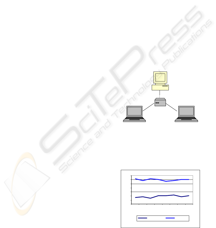
Figure 2 illustrates hardware architecture used
during evaluation of DSDW(l/t). On first computer
we place Oracle 10g with the designed database,
RMI server SDWServer and the SDW(1/t) for
managing queries. On the separate computer we
place mobile objects because they do not consume
much of the computation power and many processes
can be run simultaneously. On the last computer we
run only the Gorder service for better evaluation
time.
SDW(l/t)
SDWServer
Oracle 10g
100 Mb/s
Mobile
Object
Simulators
Gorde
r
Service
Figure 2: Testing architecture DSDW(l/t).
6.2 Single Query Experiments
30
35
40
45
50
55
60
65
2 4 6 8 10 15 20 50
Value of k
Time [ms]
Energy meters All meters
Figure 3a: Effect of value k SDW(l/t).
ICEIS 2007 - International Conference on Enterprise Information Systems
134
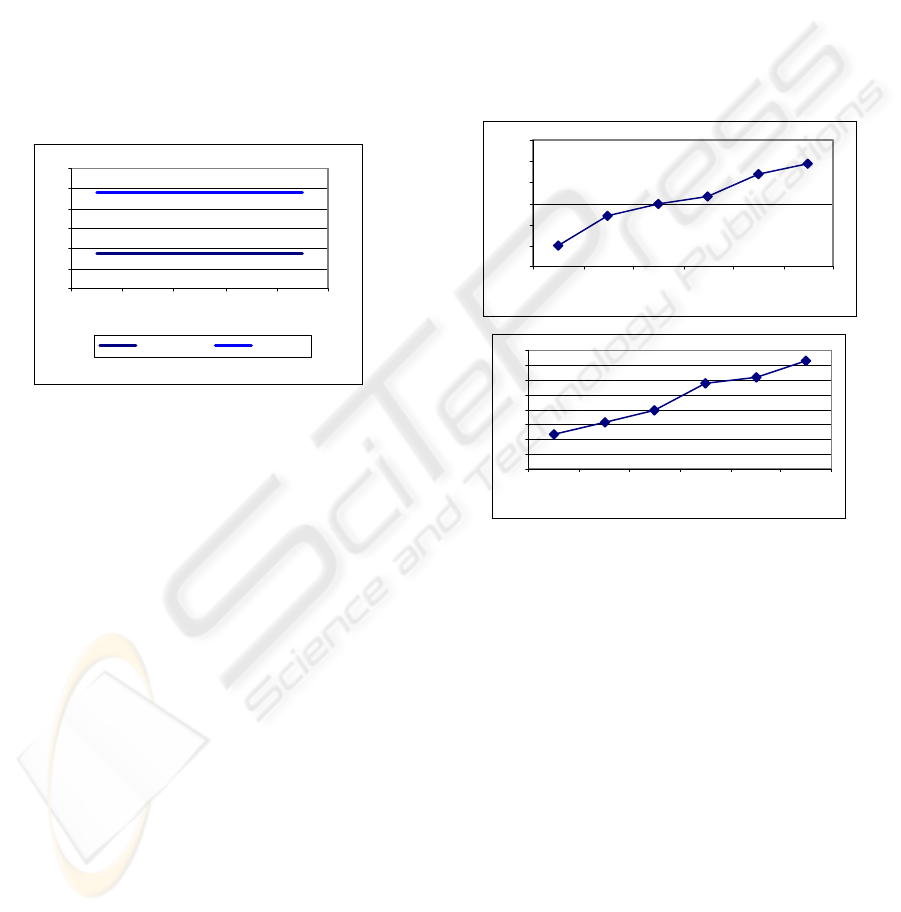
For a single query experiments we define one
mobile object. Figure 3a. illustrates that average
evaluation time of a query concerning one type of
meters (1) is more or less on constant level for non-
distributed version SDW(l/t). We can notice
distractions for k equal 6 or 8 but this aberrations are
very small, measured in milliseconds. For query
encompassing all meters (2), for higher number of
meters, an average query evaluation time increases
with the growth of value k starting from value 8,
where minimum is achieved. However, this increase
is also measured in milliseconds. For DSDW(l/t) we
can observe a little higher average measure time, but
it is constant and it does not change with the
increase of value k.
30
40
50
60
70
80
90
1 5 10 25 50
Value of k
Time [ms]
Energy meters All meters
Figure 3b: Effect of value k DSDW(l/t).
While testing the influence of of the number of
meters on query evaluation time we set parameter k
to value 20 (Figure 4). Performed experiments show,
that with the growth of number of meters the query
evaluation time increases. However, time does not
grow up very quickly. After increasing the number
of meters six times, query evaluation time increased
for about 77 % for non-distributed SDW(l/t). For
DSDW(l/t) we can notice little higher average
evaluation time. That is caused by the need of
downloading all meters data to another computer.
6.3 Simultaneous Queries Experiments
The time of full Gorder process was measured
during experiments for simultaneous queries. It
means that we measured the average summary
evaluation time for all defined queries that are
processed during single run of Gorder process.
Figure 5 summarizes the effect of number of
simultaneous queries on average Gorder process
evaluation time. All queries were defined for the
same type of meters. That is why the evaluation time
of one cycle of the Gorder process was evaluated
during one single call of the Gorder algorithm.
Concurrently with previous results, the influence of
k value on the process evaluation time is
insignificant. However, with the growth of number
of simultaneous queries the time of conducted
computations increases. For SDW(l/t) experiments
were performed only for 5 mobile objects due to
high CPU usage caused by running entire system on
one computer. It was needless to run experiments
for a greater number of mobile objects. An average
evaluation time increases with the growth of number
of queries. Each additional query causes time growth
for about 10 ms. For distributed version of the
system we could process 12 objects and more. An
average evaluation time is little higher but it is more
constant and increases slowly.
30
40
50
60
70
80
90
50 100 150 200 250 300
Number of meters per 100 km^2
Time [ms]
0
20
40
60
80
100
120
140
160
50 100 150 200 250 300
Nu mb er o f meters p er 100 km^ 2
Time [ms]
Figure 4: Effect of number of meters per 100 km
2
–
SDW(l/t) (first figure) and DSDW(l/t) (second figure).
Differentiation of queries (Figure 6) caused that
in every single cycle of Gorder process, Gorder
algorithm was called separately for every type of
query. Therefore, for four queries about four
different types of meters Gorder process called
Gorder algorithm four times. Given results for non-
distributed SDW(l/t) proved that with the growth of
the number of differential queries, process
evaluation time increases significantly. We
processed only three queries with input datasets with
the same size.
In the DSDW(l/t) we performed experiments for
12 queries. 3 queries about water meters, 3 about gas
meters and 3 about electricity meters. Each of them
with the same input dataset size. We also added 3
queries encompassing all meters. By adding queries
successively, one by one, from each type of query,
we measured average evaluation time of the entire
DISTRIBUTED APPROACH OF CONTINUOUS QUERIES WITH KNN JOIN PROCESSING IN SPATIAL DATA
WAREHOUSE
135
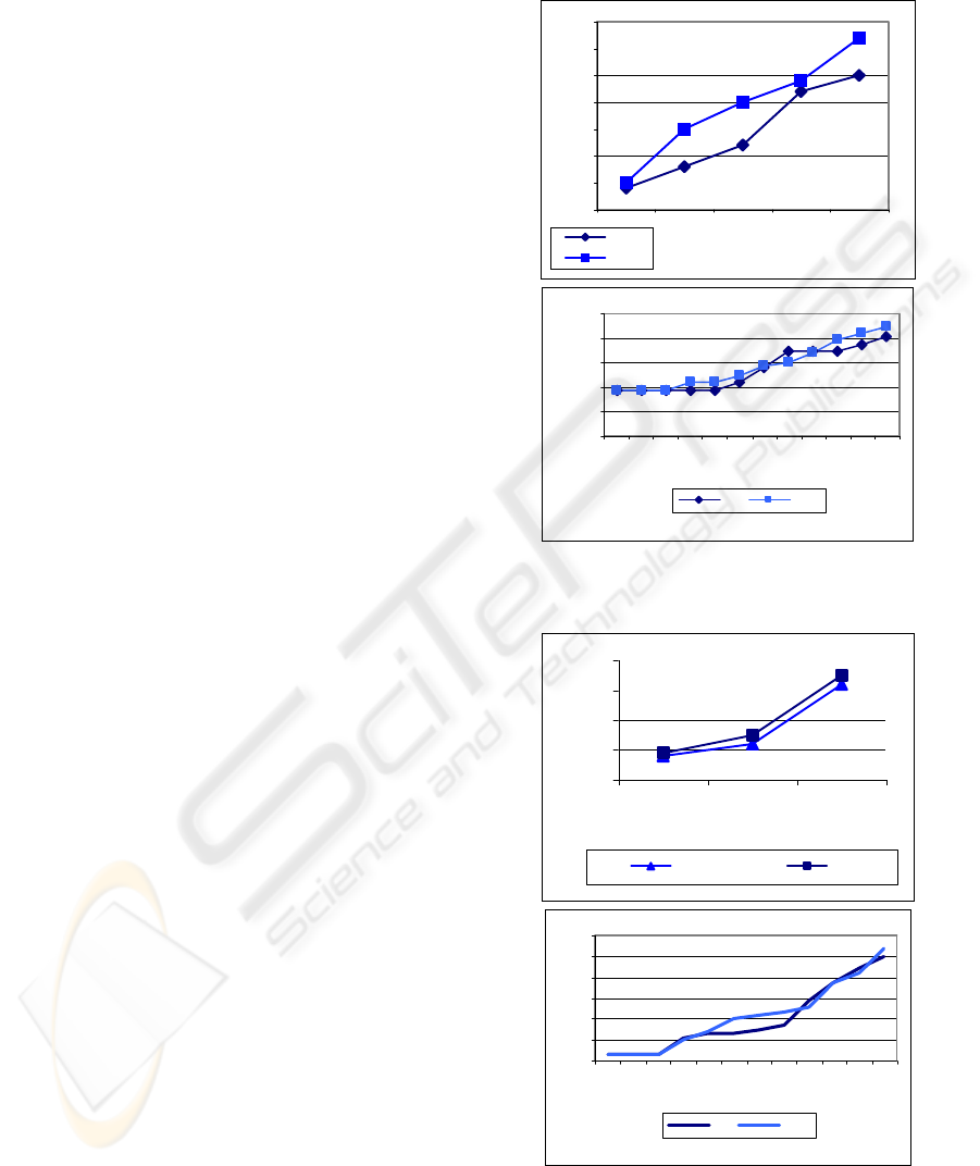
process. Given results show that with the growth of
the number of different queries the average
evaluation time increases slowly. The growth is
much less significant than in non-distributed version
and we are able to process much more queries.
7 SUMMARY
Pilot system SDW(l/t) is being improved in terms of
searching for new simultaneously continuous queries
processing techniques. Distributed approach of
designed system DSDW(l/t) shows that this
development direction should be considered for
further analysis. Furthermore, using incremental
execution paradigm as the way to achieve high
scalability during simultaneous execution of
continuous spatio-temporal queries should be
considered. Queries should be grouped in the unique
list of continuous, spatio-temporal queries, so that
spatial join could be processed between moving
objects and moving queries.
We also consider implementing solution for
balanced, simultaneous and distributed query
processing to split execution of queries of the same
type on different computers, depending on their
CPU usage prediction.
REFERENCES
Yiu, M., Papadias, D., Mamoulis, N., Tao, Y.. Reverse
Nearest Neighbors in Large Graphs. IEEE
Transactions on Knowledge and Data Engineering
(TKDE),18(4), 540-553, 2006.
Mouratidis, K., Yiu, M., Papadias, D., Mamoulis, N.,
2006. Continuous Nearest Neighbor Monitoring in
Road Networks. To appear in the Proceedings of the
Very Large Data Bases Conference (VLDB), Seoul,
Korea, Sept. 12 - Sept. 15, 2006.
Gorawski M., Wróbel W., 2005. Realization of kNN Query
Type in Spatial Telemetric Data Warehouse. Studia
Informatica, vol.26, nr 2(63), pp.1-22, 2005.
Gorawski M., Malczok R., 2004. Distributed Spatial Data
Warehouse Indexed with Virtual Memory Aggregation
Tree. 5th Workshop on Spatial-Temporal DataBase
Management (STDBM_VLDB’04), Toronto, Canada
2004.
Chenyi Xia, Hongjun Lu, Beng Chin Ooi, Jing Hu, 2004.
GORDER: An Efficient Method for KNN Join
Processing, VLDB 2004, pp. 756-767.
Böhm Ch., Braunmüller B., Krebs F., Kriegel H., 2001.
Epsilon Grid Order: An Algorithm for the Similarity
Join on Massive High-Dimensional Data, Proc. ACM
SIGMOD INT. Conf. on Management of Data, Santa
Barbara, CA, 2001.
Hammad M. A., Franklin M. J., Aref W. G., Elmagarmid
A. K., 2003. Scheduling for shared window joins over
data streams. VLDB, 2003
50
55
60
65
70
75
80
85
12345
Number of simultaneous queries
Time [ms]
k = 5
k = 10
40
60
80
100
120
140
123456789101112
Number of simultaneous queries
Time [ms]
k=5 k=10
Figure 5: Effect of number of simultaneous queries –
SDW(l/t) (first figure) and DSDW(l/t) (second figure).
40
50
60
70
80
123
Number of different simultaneous queries
Time [ms]
k = 5 k=10
40
60
80
100
120
140
160
123456789101112
Number of simultaneous queries
Time [ms]
k=5 k=10
Figure 6: Effect of differentiation of simultaneous queries
– DSDW(l/t).
ICEIS 2007 - International Conference on Enterprise Information Systems
136
