
NEURAL NETWORKS FOR DATA QUALITY MONITORING OF
TIME SERIES
Augusto Cesar Heluy Dantas and Jos
´
e Manoel de Seixas
Signal Processing Lab, COPPE/EP - Federal University of Rio de Janeiro, C.P. 68504, Rio de Janeiro 21945-970, Brazil
Keywords:
Data Quality, Feed-Forward and Recurrent Neural Networks, Time Series, Monitoring System.
Abstract:
Time series play an important role in most of large data bases. Much of the information comes in temporal
patterns which is often used for decision taking. Problems with missing and noisy data arise when data
quality is not monitored, generating losses in many fields such as economy, customer relationship and health
management. In this paper we present a neural network based system used to provide data quality monitoring
for time series data. The goal of this system is to continuously adapt a neural model for each monitored series,
generating a corridor of acceptance for new observations. Each rejected observation may be substituted by
its estimated value, so that data quality is improved. A group of four diverse time series was tested and the
system proved to be able to detect the induced outliers.
1 INTRODUCTION
Technology and scientific research are becoming
more and more “data driven”, and specialists say that
this century is surely the century of data (Donoho,
2000). For example, the poor quality of customer
data costs U.S. business more than US$600 billion
per year (Eckerson, 2001). It is then easy to see that
data are critical assets in the information economy,
and that the quality of the data from a company or
research center is a good predictor of their future suc-
cess.
Time series data are some of the most common
types of data involved in information systems. Much
of the data stored in nowadays databases come in
temporal patterns which are important sources of
knowledge. The development of time series fore-
casting methods is gaining importance as companies
and research centers give more emphasis to a data
based knowledge and make their investments in a data
driven way. Neural networks have been successfully
applied to the task of modeling time series, specially
since the end of the 1980’s (Kaastra and Boyd, 1996).
As the amount of data in such data bases increases
exponentially, a Data Quality Monitoring System may
be of crucial importance to maintain data free-of-
error. In this context, we propose a neural network
based system to treat time series data. The monitor-
ing system should be able to detect faults in data (such
as outliers and missing values) and replace them by
accurate estimates.
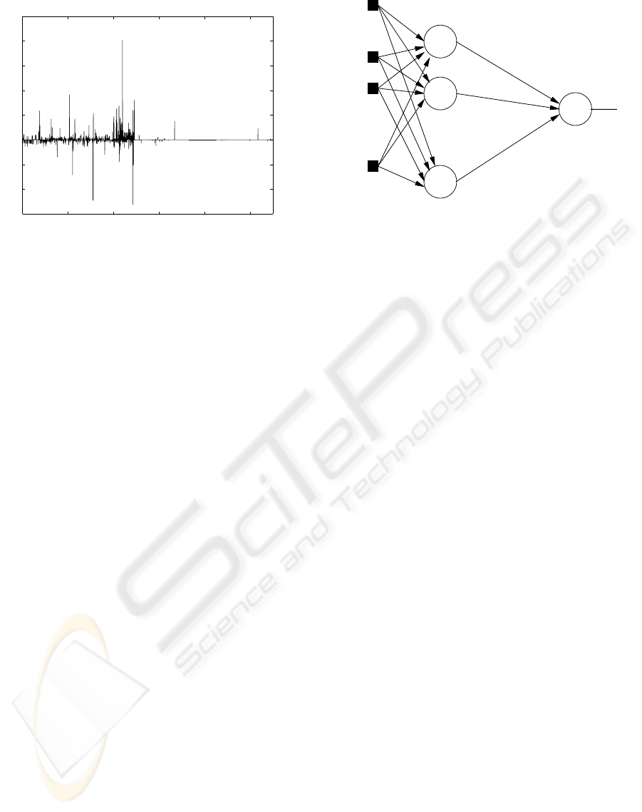
As an example of the importance of monitoring
data quality, we show in Figure 1 the difference be-
tween two series that intend to represent the same in-
formation, that is, the AMD (Advanced Micro De-
vices Inc.) stock value at the end of each day. The cer-
tified series was obtained from Stockwiz (Stockwiz,
2006), and the non-certified series was freely down-
loaded from Yahoo!Finance (Yahoo!Finance, 2006).
We may note that Yahoo!Finance has clearly im-
proved its data quality by the end of the year 2000,
following a global tendency of applying efforts to as-
sure a minimum of data quality. However, free data
will never offer the same guarantee of being free-of-
error like certified data and must always be analyzed
before use.
The aim of this work is not to develop a predic-
tion algorithm; actually, what we propose is a sys-
tem that monitors the quality of time series data by
drawing reliability regions (corridors of acceptance)
from the predicted values. The monitoring system is
designed to operate in accordance to a human super-
411
Cesar Heluy Dantas A. and Manoel de Seixas J. (2007).
NEURAL NETWORKS FOR DATA QUALITY MONITORING OF TIME SERIES.
In Proceedings of the Ninth International Conference on Enterprise Information Systems - AIDSS, pages 411-415
DOI: 10.5220/0002371004110415
Copyright
c
SciTePress
1996 1998 2000 2002 2004 2006
−15
−10
−5
0
5
10
15
20
25
Days (from Jan−19−1996 to Sep−01−2006)
Difference between Certified and Non−Certified Series (%)
Figure 1: Percentage differences between certified and non-
certified AMD data along the years.
visor, who may validate or not the system automatic
decisions (Dantas and Seixas, 2005).
In the next section, we give a brief description of
some time series data quality issues. In Section 3,
we summarize the neural networks methods used in
the system developed for time series modeling. The
complete monitoring system is presented in Section 4.
Some application examples are detailed in Section 5,
and the conclusions are addressed in Section 6.
2 DATA QUALITY ISSUES FOR
TIME SERIES
We may define Data Quality (DQ) as follows: data
has quality if it satisfies the requirements of its in-
tended use, that is, if it has conformity to the specifi-
cations (Olsen, 2003).
Of course, this definition is closely related to the
accuracy dimension, meaning that more accurate data
have always a greater quality. On the other hand, it
does not mean that not so accurate data have necessar-
ily low quality. For example, a 90% accurate database
may be considered to have a poor data quality if one
intends to use it in a high security purpose, but this
same data may be viewed as high quality data if its
intended use relates to finding potential costumers of
a new product.
Timeliness (how up-to-date is your database?) and
completeness (does your database have missing val-
ues?) dimensions are also taken into account in our
monitoring system.
1
x
t−N +1
˜x
t+F
...
...
w
HN
v
1
v
H
b
1
x
t−1
x
t
Figure 2: Feed-forward scheme for predicting future data.
3 NEURAL NETWORK
ARCHITECTURES
The developed system works with two types of neu-
ral networks: feed-forward with back-propagation
(FFBP) training algorithm (Haykin, 1999) and recur-
rent Elman network (Elman, 1990). The choice for
the architecture to be used is also data driven, that is,
for each analyzed time series we test the accuracy of
both models and choose the best.
Figure 2 shows in a simple way the prediction
scheme used with a feed-forward network. To form
the input vector, we first analyze the autocorrelation
plot of the whole (pre-processed) training series and
then choose all the N past lagged observations that
proved to have significant correlation with the refer-
ence observation. The hidden layer contains H biased
neurons with the hyperbolic tangent as the activation
function. For the output layer, we use a non-biased
linear neuron for x
t+F
estimation. In this work, the
lag F is always one, but generalization for larger hori-
zons of prediction is straightforward. These predic-
tions form an “uncertainty cone” (the corridor), inside
which the new observations must lay to be accepted as
valid data.
Figure 3 illustrates the generic architecture of an
Elman recurrent network. The main difference with
respect to the FFBP scheme is that Elman networks
have a feedback loop in the hidden layer, which al-
lows all the past observations to contribute to the de-
termination of the future ones.
4 THE MONITORING SYSTEM
As previously mentioned, the goal of the monitoring
system is not to provide data prediction, but to per-
form a validation test to accept or reject (with the
ICEIS 2007 - International Conference on Enterprise Information Systems
412

.
.
.
p
Input Recurrent tanh layer Output linear layer
D
b
1
a
2
(k) = y
a
2
(k) = LW
2,1
a
1
(k) + b
2
a
1
(k) = tanh(IW
1,1
p + LW
1,1
a
1
(k − 1 + b
1
))
a
1
(k − 1)
b
2
a
1
(k)
11
IW
1,1
LW
1,1
LW
2,1
.
Figure 3: Elman network generic structure.
proper correction), if desired, any new observation of
the monitored time series.
Data Monitoring comprises two main phases. In
the first one (which is an off-line phase), a sufficient
number of past observations of the series are used
to adjust a pre-processing algorithm, that will be de-
scribed in the next subsection. These pre-processed
observations are then used to train a neural forecast-
ing model, using both feed-forward and recurrent net-
work architectures as described in the previous sec-
tion. The trained neural model is considered to be
adjusted when the forecasting error for the test set
(composed by the last observations of the available
data) lay within a previously specified value for the
individual time series under analysis. In this phase,
the error figure used is the MAPE (Medium Absolute
Percentage Error).
The second phase works on-line. Each monitored
series has already had an adjusted model ready to re-
ceive a new observation and to test its validity. This
validation test will be detailed in the subsection 4.2.
4.1 Semi-automatic Pre-processing
Algorithm
The pre-processing phase has a great importance and
much of the monitoring success depends on it.
First of all, one must detect if the time series trend
is stochastic or deterministic. We perform this ver-
ification by applying a combination of Augmented
Dickey-Fuller (ADF) (Dickey and Fuller, 1979) and
Phillips-Perron (Phillips, 1987) tests. The resulting
test detects whether or not there are unit roots in the
generating process of the time series. If they exist, it
means that the trend is stochastic and that one must
take the first difference of the series n times in order
to make it stationary, being n the number of unit roots
detected (that is, the order of integration of the pro-
cess).
If the test detects no unit roots, one may conclude
that the trend is deterministic. In this case, we remove
the trend by performing a polynomial fitting. In both
stochastic or deterministic cases, we also test for the
presence of seasonal cycles (after trend removing), re-
N
greater than zero?
of unit roots
Is the number "n"
Verify the presence of any cycles
and remove them by spectral (FFT)
analysis or periodic diffrencing
Series is now pre−processed and
ready to be fed into the neural system
of the series "n" times
Take the first difference
Set "Stochastic Trend" flag "On"
Set "Deterministic Trend" flag "On"
Remove the series trend
by polynomial fitting
Perform Unit Root Test
Select a series
Y
Figure 4: Semi-automatic pre-processing algorithm to re-
move trends and possible cycles.
moving them by spectral (Fourier) analysis or by a
convenient periodic differences
1
(Chatfield, 1984).
This pre-processing phase is claimed to be semi-
automatic because it cannot exclude the intervention
of a human specialist, who inserts his or her knowl-
edge into the system, mainly for cycles removing.
Figure 4 shows these steps in a flow diagram.
4.2 Validation Test
The on-line phase of the monitoring system consists
of receiving new observations and testing their va-
lidity according to the previously developed model.
When a new observation x(T) arrives, we have al-
ready an estimated (predicted) value for it (ˆx(T)),
which was determined by the adjusted neural model.
Here, human intervention may also be necessary.
For example, new observations can be excluded by
direct action of a manager who feels that they are bi-
ased by some temporary condition that he or she is
aware of (and that the system cannot be able to track
on time). On the other hand, the system is designed to
automatically screen all current observations to iden-
tify those that appear unusual, that is, outliers. Each
outlier could be called to the attention of an appro-
priate management person, who would then decide
whether or not to include the observation in the fore-
casting process (Montgomery et al., 1990). In fact,
this outlier may have a reasonable origin, or may sim-
ply be the result of error.
Outliers can be identified by analyzing the fore-
cast error e(T) = x(T) − ˆx(T). If this error is large,
it may be concluded that the observation x(T) came
1
If a series is known to have a weekly seasonality (as
the case of electricity consume), it is more convenient to
remove this cycle by applying the (1− B
7
) operator, where
B is the delay operator, that is, Bx(t) = x(t −1).
NEURAL NETWORKS FOR DATA QUALITY MONITORING OF TIME SERIES
413
0 100 200 300 400 500 600 700
0
5
10
15
(a)
0 50 100 150 200 250 300 350 400
1
2
3
4
x 10
5
(b)
0 200 400 600 800 1000 1200 1400 1600 1800
20
30
40
50
(c)
0 100 200 300 400 500 600
1.5
2
2.5
3
x 10
5
(d)
Figure 5: Series used to test the system: (a) Monthly USA
civilian unemployment, from 1952/Jan to 2006/Aug; (b)
Monthly Electricity consume in USA, from 1973/May to
2006/Aug; (c) Daily SUN close stock values, from 1998/Jan
to 2002/Dec and (d) Monthly USA total population, from
1952/Jan to 2006/Aug.
from a different process. The test for outliers may
logically take the form
|
e(T)
ˆ
σ
e
|> K (1)
where K is typically 4 or 5 (for outlier detection). In
this paper, we used K = 4, in order to achieve a more
restrictive filtering of the time series. So, the width
of the corridor to detect outliers is 4
ˆ
σ
e
, where
ˆ
σ
e
is
dynamically updated.
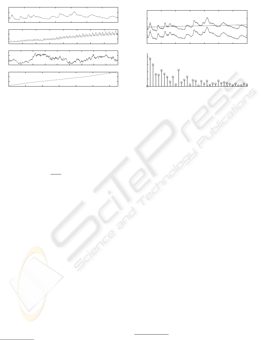
5 SOME STUDY CASES
We tested the system for several real time series data,
representing various kinds of processes. In this sec-
tion, we summarize some of the obtained results. Out-
liers and missing values
2
were artificially introduced.
Figure 5 shows four series used to test the
monitoring system: USA civilian unemploy-
ment (Economagic, 2006), USA Total Electricity
Consume (Economagic, 2006), SUN Microsystems
Stock Close Value (Stockwiz, 2006) and Total USA
Population (Economagic, 2006). The process of
removing trend and cycles is illustrated in Figure 6
for the unemployment series.
Training the neural models showed that an FFBP
network with 8 hidden neurons (h. n.) achieves the
2
As all the tested series are always greater than zero,
missing values were induced by introducing zeros in the se-
ries.
0 100 200 300 400 500 600 700
−5
0
5
10
15
Months (from 1952/Jan to 2006/Aug)
Unemployment
0 0.01 0.02 0.03 0.04 0.05
0
100
200
300
400
Normalized Frequency
Magnitude
Cycle 1
Cycle 2
Cycle 3
Figure 6: Removing trend and cycles from the unemploy-
ment series.
best MAPE (2.49%) for this series, while an Elman
network achieves 2.66%. This was the only case
where Elman MAPE was found (slightly) larger than
FFBP one. Figure 7 shows the application of the
monitoring system to the test series (last 40 observa-
tions of the total series, not seen by the neural model).
Three outliers were introduced and correctly removed
and substituted by the estimated values
3
, while none
of the series original points was rejected. The visual-
ized corridor is suitable to detect outliers without re-
jecting extreme (but correct) values. Note that it was
possible to correctly reject the third outlier because of
the accuracy of the estimated series, which made that
the corridor of acceptance did not reach the outlier.
This same experiment was performed for the remain-
ing series under test.
Table 1 summarizes the obtained results.
6 CONCLUSIONS
The relevance of monitoring systems to assure data
quality through fault detection and correction was
stated. By online filtering outliers and replacing miss-
ing values, the proposed neural system works towards
increasing the most important data quality issues (ac-
curacy, timeliness and completeness), by substituting
each wrong observation or filling each missing data
by a proper estimated value.
Results demonstrated the tendency for Elman net-
works outperforming the FFBP ones. This is due to
3
Of course, a false point that felt inside the corridor of
acceptance would not be removed by the semi-automatic
algorithm. It could not be treated as an outlier by the system
and should be detected by another technique.
ICEIS 2007 - International Conference on Enterprise Information Systems
414
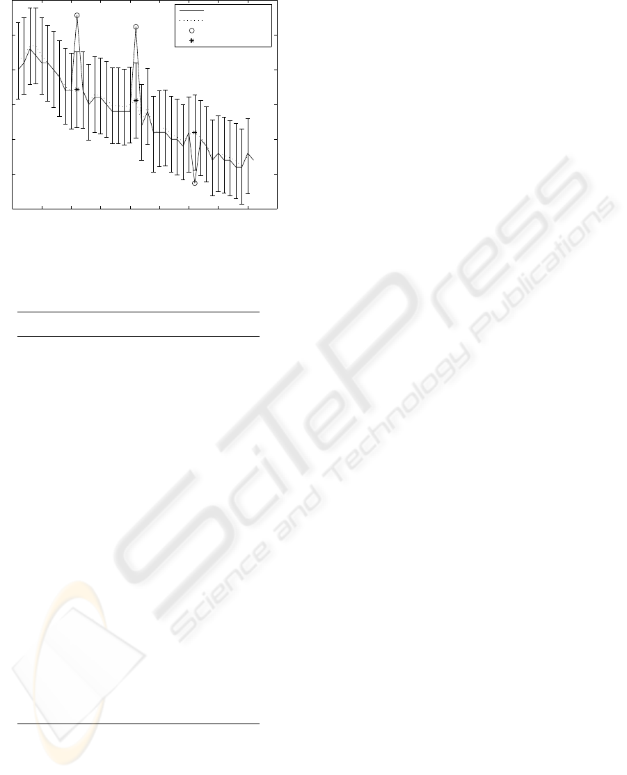
0 5 10 15 20 25 30 35 40 45
4
4.5
5
5.5
6
6.5
7
Months (from 2003/May to 2006/Aug)
Civilian Unemployment Rate (Percent)
Corridor of Acceptance
Received Series
Estimated Series
Detected Outliers
Replaced Values
Figure 7: Monitoring the test series of unemployment.
Table 1: Summary results for some of the tested series.
Series Name Features
USA Unemployment
Frequency Monthly
Trend Deterministic (linear)
Cycles four low frequency
Neural Network 8 h. n. FFBP
MAPE 2.49%
Electricity Consume
Frequency Monthly
Trend Deterministic (linear)
Cycles three
Neural Network 6 h. n. Elman
MAPE 4.01%
SUN Stock
Frequency Daily
Trend Stochastic (n = 1)
Cycles two low frequency
Neural Network 4 h. n. Elman
MAPE 1.81%
USA Population
Frequency Monthly
Trend Stochastic (n = 1)
Cycles three low frequency
Neural Network 8 h. n. Elman
MAPE 0.74%
the feedback loop in the hidden layer, which facili-
tates the detection of temporal patterns. This moni-
toring system should then be used as a support tool to
perform online filtering when acquiring non-certified
time series data, or to scan databases searching for
outliers and appropriately completing the missing val-
ues.
ACKNOWLEDGEMENTS
We would like to thank CNPq and FAPERJ (Brazil)
for their support to this project.
REFERENCES
Chatfield, C. (1984). Analisys of Time Series. Chapman and
Hall.
Dantas, A. C. H. and Seixas, J. M. (2005). Adaptive
neural system for financial time series tracking. In
Ribeiro, B., editor, ICANNGA - International Con-
ference on Adaptive and Natural Computing Algo-
rithms, Springer Computer Series: Adaptive and Nat-
ural Computing Algorithms, pages 421–424. Elsevier.
Dickey, D. A. and Fuller, W. A. (1979). Distributions of the
estimators for autoregressive time series with a unit
root. Journal of the American Statistical Association,
75:427–431.
Donoho, D. L. (2000). High-dimensional data analysis: The
curses and blessings of dimensionality. Lecture for the
American Math. Society “Math Challenges of the 21st
Century”.
Eckerson, W. W. (2001). Data quality and the bottom line.
Technical report, The Data Warehousing Institute.
Economagic (2006). Economagic web site.
www.economagic.com.
Elman, J. L. (1990). Finding structure in time. Cognitive
Science, 14:179–211.
Haykin, S. (1999). Neural Networks - a Comprehensive
Foundation. Prentice-Hall, 2nd. edition.
Kaastra, I. and Boyd, M. (1996). Designing a neural net-
work for forecasting financial and economic time se-
ries. In Neurocomputing, number 10, pages 215–236.
Elsevier.
Montgomery, D. C., Lynwood, A. J., and Gardner, J. S.
(1990). Forecasting and Time Series Analysis.
McGraw-Hill.
Olsen, J. E. (2003). Data Quality: the Accuracy Dimension.
Morgan Kaufmann Publishers.
Phillips, P. C. B. (1987). Time series regression with a unit
root. Econometrica, 55(2):277–301.
Stockwiz (2006). Stockwiz web site. www.stockwiz.com.
Yahoo!Finance (2006). Yahoo!Finance web site.
http://finance.yahoo.com.
NEURAL NETWORKS FOR DATA QUALITY MONITORING OF TIME SERIES
415
