
GRID WORKFLOW SCHEDULING WITH TEMPORAL
DECOMPOSITION
∗
Fei Long and Hung Keng Pung
Network Systems and Services Lab., Department of Computer Science, National University of Singapore, Singapore
Keywords:
Grid Workflow, Scheduling, Decomposition, QoS.
Abstract:
Grid workflow scheduling, a very important system function in current Grid Systems, is known as a NP com-
plete problem. In this paper, we propose a new scheduling method– “temporal decomposition” – which divides
a whole grid workflow into some sub-workflows. By dividing a large problem (workflow) into some smaller
problems (sub-workflows), the “temporal decomposition” to better exploit achieves much lower computation
complexity. Another motivation for the design of “temporal decomposition” is at the availability of the highly
dynamic grid resources. We further propose an efficient scheduling algorithm for scheduling sub-workflows
in this paper. Numerical simulation results show that our proposed scheme is more efficient in comparison
with a well known existing grid workflow scheduling method.
1 INTRODUCTION
The grid workflow has some unique characteristics
which are different from conventional workflow, such
as business workflow(Zhang et al., 2004). These
characteristics include: 1) Highly dynamic grid re-
sources. Unlike in traditional workflow systems, re-
sources in grid network can join and leave the net-
work at any time, e.g. during the execution of as-
sociated grid tasks. Such changes of resource quan-
tity may lead to cause the failure of task execution
or even locked situation. 2) Distributed characteris-
tic. In conventional workflow system, the resources
are concentrative and managed in centrally concen-
trative way. However, both resources and resource
management system (RMS) are distributed in current
grid networks. Thus it is impossible to obtain global
resources information for a single request. 3) Uncer-
tain execution time. Due to the variance in assigned
resource, the execution time of each grid task is un-
certain. Furthermore, the capacity of each resource
in the grid network is highly diverse, which makes
the execution time different even for the same task
∗
The work is funded by SERC of A*Star Singapore
through the National Grid Office (NGO) under the research
grant 0520150024 for two years.
assigned to different resources. Due to these factors,
the conventional workflow management system can’t
be applied to grid environment directly. A new grid
workflow scheduling algorithm is clearly desirable.
In this paper, we propose a new distributed workflow
scheduling algorithm for p2p grid network.
It is well known that the scheduling of grid work-
flow to distributed grid resources is a NP-complete
problem. One effective way to solve such problem
is to divide a big problem into some smaller sub-
problems. Thus decomposition of workflow is mean-
ingful for solving grid workflow scheduling prob-
lem. Besides space decomposition(Yu et al., 2005)
of workflow, which divides the workflow into some
parts according to the workflow structure and rela-
tionships between tasks, in this paper we present an-
other method of dividing grid workflow into smaller
parts; it is known as temporal decomposition. Tem-
poral decomposition divides workflow according to
the estimated start time of a task and its execution
dependencies with other between tasks. Suppose
the scheduler is scheduling tasks starting from time
t
0
. Only the tasks whose preceeding tasks have all
finished or running, and whose start times are less
than the t
0
+ “scheduling window”(an important sys-
tem parameter) will be considered in current schedul-
441
Long F. and Keng Pung H. (2007).
GRID WORKFLOW SCHEDULING WITH TEMPORAL DECOMPOSITION.
In Proceedings of the Ninth International Conference on Enterprise Information Systems - ISAS, pages 441-446
DOI: 10.5220/0002373904410446
Copyright
c
SciTePress

ing decision.
Our main contributions in this paper are two fold-
ers. First, we use temporal decomposition to reduce
the complicated grid workflow scheduling problem
to simplified the scheduling of sub-workflow (paral-
lel tasks), which is easier to solve and realized. Sec-
ondly, we propose an efficient on-line scheduling al-
gorithm for the decomposed sub-workflows. By using
a QoS bidding mechanism, this scheduling algorithm
can find the near-minimum cost decision without vio-
lations of QoS constraints.
This paper is organized as follows. In Section 2,
we present some important existing grid workflow
scheduling heuristics. Section 3 presents the system
model used in this work. Our proposal is introduced
in Section 4. Section 5 presents some simulation re-
sults which demonstrate the effectiveness of our pro-
posal. Finally, we conclude this work paper in Sec-
tion 6.
2 WORKFLOW
DECOMPOSITION
One possible method for solving NP-complete prob-
lem is to divide a big problem into some small
problems, since the computation complexity de-
creases dramatically with the problem size. Thus
the approach of decomposition of workflow struc-
ture is an attractive approach for solving grid
workflow scheduling problem. There are two
different approaches to de-compose the workflow
structure– “space decomposition” and “level decom-
position”(Deelman et al., 2004). “Space decompo-
sition” divides the workflow into some parts accord-
ing to the workflow structure and relationships be-
tween tasks. For example, Yu(Yu et al., 2005) di-
vides workflow into independent branches and syn-
chronization tasks, and schedules these branches or
synchronization tasks separately. A synchronization
task is defined as a task with multiple preceding tasks
or succeeding tasks, while the task with only one or
less preceding task and succeeding task is called sim-
ple task. A branch contains a series of simple tasks
executed sequentially between two synchronization
tasks. The decomposition result of “space decompo-
sition” is highly dependent on the workflow structure.
For example, there are many synchronization tasks in
a workflow with small number of serial tasks. The
scheduling for synchronization task is far from opti-
mal since only one task has been considered.
A simple “level decomposition” method has been
proposed in(Deelman et al., 2004) . In such decompo-
sition method, the abstract workflow is decomposed
into some sub-workflows, which consist of tasks with
the same level (determined by the execution depen-
dency) in the abstract workflow structure. The new
sub-workflows will be submitted to a scheduler, and
the scheduler will make decision based on all tasks
in a sub-workflow together instead of individual task.
“Level decomposition” is too simple to support com-
plicated workflow components, such as loop task.
Another shortcoming of “level decomposition” is that
the next-level sub-workflow will not start to execute
until all tasks in previous-level sub-workflow have
been completed.
3 SYSTEM MODELS
In this paper, we adopt the definition of grid workflow
as an abstract representation of application running on
grid networks. Grid workflow is a set of tasks that are
executed on multi-sited grid resources in a specific
pre-defined order(Yu and Buyya, 2005). Grid tasks
are the atomic level components in the grid workflow.
These components are independently executed on lo-
cal grid resources. The abstract grid tasks may rep-
resent various application components, such as MPI
tasks which can execute on multiple processors. Thus,
these tasks have various QoS requirements, which
could be satisfied by choosing good schedules with
appropriate resource mapping. The typical QoS met-
rics used in grid networks includes(Cardoso et al.,
2004): time (deadline), cost (budget), and reliability.
As the basic and most important performance metric,
“time” refers to the finish time of whole workflow ex-
ecution. The usage of grid resources will be charged
by the resource owner, if the resource does not belong
to the user submitting the workflow. Furthermore, the
cost of managing workflow in grid system should also
be paid born by the users. The execution of grid tasks
is depend on the availability and reliability of the re-
sources. For example, when a resource leaves the grid
system, all tasks running on it will fail and should be
re-executed on another resource.
3.1 Qos Bid Model
Suppose there are M distributed resources in the sys-
tem. All resources support resource conservation with
a limited amount of processing capacity. The capaci-
ties of resources are represented by {c
i
}, i = 1, . . . , M,
which may have different definitions (e.g. number
of processors, CPU cycles, memory size). These re-
sources are shared among the end-users with different
QoS requirements. There is a local agent (LA) for
each resource as shown in Figure 1.
ICEIS 2007 - International Conference on Enterprise Information Systems
442

Cluster
LA 1
LA n
LA 2
P2P Grid Network
Req
Bid
Req
Bid
Workflow Req
User
Cluster
Figure 1: Grid Framework.
Each LA can play one of two roles– as a scheduler
or a contractor. A scheduler LA collects the work-
flow requests from end-users, and is responsible for
scheduling the workflow to distributed resources. The
contractor LA is referred to the LA which accepts task
from the scheduler LA and performs local scheduling,
runtime state monitoring and etc. The roles of LAs
are not fixed and are not pre-defined in advance. In
fact, these roles are dynamically changed by the re-
quirement of users. Therefore, a LA may alternate
between two roles or maintain both roles in the same
time during the system operation.
When a workflow request arrives at the scheduler
LA, the LA will at first analyze the structure of work-
flow and de-composite the workflow into tasks. The
individual QoS requirements of each task will be de-
rived from the QoS requirement of whole workflow.
Each task has its own QoS requirement and capacity
requirement, represented by q
j
and r
j
(j = 1, . . . , N)
respectively. The QoS requirement typically has a
tolerance bound, which is presented by a percent-
age value b
j
. In other words, the bound for QoS re-
quirement is q
j
(1± b
j
). Then the LA will query the
available resources by broadcast the query message to
neighborhood contractor LAs, which can receive the
broadcast message. After receiving the query mes-
sage, the neighborhood LAs will check their available
resources capacity and compare it to the QoS require-
ment of the task. If the QoS requirement of the task
can be satisfied, the contract LA will quote a price and
send back its bid to the scheduler LA. The query mes-
sage contains two important time information– dead-
line of this task and life time of this query message;
the latter indicates the longest resource query time for
this task. In other words, the contractor LA should
reply within the life time, otherwise the reply will be
viewed as expired.
The QoS bids for one task will be stored in an indi-
vidual bid queue. All tasks have their own bid queues.
The order of bids in the queue can be adjusted by the
scheduler. The scheduler will choose a bid for each
task in the sub-workflow. The set of selected bids for
the sub-workflow constitutes the schedule decision.
3.2 Workflow Model
The previous work on grid workflow model can be
classified to two types– abstract and concrete. In
the abstract model, grid workflow is defined without
referring to specific grid resources. In the concrete
model, the definition of workflow includes both work-
flow specification and related grid resources. Defin-
ing a new model for scientific grid application is be-
yond the scope of this paper. We adopt the abstract
DAG model to describe grid workflow as following
definition.
Definition 1 A grid workflow is a DAG denoted by
W = {N , E }, where N is the set of grid tasks and E
the set of directed task dependencies. Let s(n), p(n)
be the sets of succeeding tasks and preceding tasks of
task n ∈ N respectively. n
s
∈ s(n) means ∃(n, n
s
) ∈ E ,
while n
p
∈ p(n) ⇐⇒ ∃(n
p
, n) ∈
E .
In this model, the grid task is an abstract defini-
tion, which can be the representation of various cate-
gories of tasks, such as data transfer task and calcula-
tion task and etc.
3.3 Optimal Objective
Price function P(i, j)(Smale, 1976)(Wolski et al.,
2001)(Cheng and Wellman, 1998) represents the cost
of executing task j at resource i. Thus, our design
objective is to minimize the total cost of workflows.
minimum
∑
P(i, j) (1)
subject to,
q
j
is satisfied∀ j
∑
j
r
j
x
i, j
< c
i
∀i, j
(2)
where
x
i, j
=
1, task j is assigned to resource i
0, else.
(3)
4 PROPOSAL
4.1 Maximum Parallel Tasks
Unlike traditional static scheduling for the whole grid
workflow, we introduce the concept of “Maximum
parallel tasks” (MPT) for decomposing workflow.
Workflow decomposition provides a feasible alterna-
tive way for reducing a large workflow scheduling
problem to some smaller sub-workflow scheduling
problems. Besides space decomposition, there is an-
other method of dividing grid workflow into smaller
GRID WORKFLOW SCHEDULING WITH TEMPORAL DECOMPOSITION
443
parts– temporal decomposition. Temporal decompo-
sition divides workflow according to the estimated
start/end time of tasks.
Another idea behind “MPT” is to reduce work-
flow scheduling problem to parallel tasks (sub-
workflow) scheduling. Different from independent
parallel tasks, tasks of grid workflow have some inter-
dependency, such as relationship of execution order
and relevancy of data. These inter-dependencies make
the workflow scheduling more complicated, since
the schedule should satisfy these dependency con-
straints. Dividing the whole workflow into sets of in-
dependent parallel tasks will convert a complex work-
flow scheduling problem to a simpler parallel tasks
scheduling problem.
We use MPT to divide the whole workflow into
some parts. Thus the scheduling problem complexity
is highly reduced due to the smaller size of MPT com-
pared to that of whole workflow. MPT is defined as
the waiting tasks which have no un-started preceding
tasks (i.e. all their preceding tasks have been com-
pleted or are running), and are within next scheduling
window. For example, currently there are three paral-
lel tasks (task T1, T2 and T3) running in the system,
as shown in Figure 2. Task T4, T5 and T6 are the
succeeding task of task T1, T2 and T3, respectively.
Suppose task T1 finishes before task T2 and T3, when
task T1 finishes, the MPT task set will be task T4, T5
and T6, because the preceeding tasks (T2 and T3) of
T5 and T6 are running and the estimated finish times
of T2 and T3 do not exceed the scheduling window.
Since task T2 and T3 are still running, task T5 and
T6 will be scheduled to start after the estimated finish
time of their preceding tasks. The big advantage of
grid computing is its parallel computation capability.
Thus we argue a grid workflow should contain a large
proportion of parallel tasks in its structure, in order to
utilize the parallel computation capability in grid sce-
nario. Therefore, the size of MPT should not be too
small (e.g. equals to 1). Furthermore, usually there
are multiple workflow requests at the same LA.
T1
T5
T2 T3
T4
T6
MPT1
MPT2
t
Figure 2: Example of maximum parallel tasks.
Scheduling window is an important design param-
eter for our system. The length of scheduling win-
dow is the space between current scheduling time and
next scheduling time. It directly determines the size
of MPT waiting to be scheduled. In other words, the
value of scheduling window is proportional with the
size of MPT. Therefore, its value should neither be too
small nor be too great. The selection of next schedul-
ing time point should consider this aspect. The selec-
tion algorithm for the next scheduling time is shown
in Algorithm 1.
Algorithm 1 Next scheduling time algorithm.
{ f
i
} ← finish times of tasks with unscheduled suc-
ceeding task(s) in current MPT
t
min
← the task with earliest finish time f
min
=
min{ f
i
}
next scheduling time ← t
min
Can MPT deal with more complex Grid Workflow
components, such as split, merge, condition, loop
task? Split component is a Grid task with multiple
succeeding tasks. Split component is fully supported
by MPT. When the split task is running or finished,
its child tasks (if they have no other preceeding task)
can be included in the next MPT and wait for schedul-
ing. As the opposite of split component, merge com-
ponent is a Grid task with multiple preceeding tasks.
It can also be supported by MPT if we introduce the
following constraint: unless all the preceeding tasks
of a merge task are running or finished, this merge
task can not be scheduled. However, this constraint
may impair the performance of scheduler, since fewer
number of tasks in the next MPT. In condition com-
ponent, one of the possible next Grid tasks is selected
based on a condition. The change of execution path
makes traditional static scheduling schemes not fea-
sible. However, MPT is constituted during run-time.
It can support condition component well by adding
condition constraint. Loop task will be iterated for
many times in a Grid Workflow. There are two kinds
of loop tasks- fixed loop and condition loop. The it-
eration times of fixed loop task is predefined and will
not change in runtime. Thus we can stretch a fixed
loop task to a sequence of tasks which is fully sup-
ported by MPT. The condition loop task’s execution
times depend on a condition expression. By adding
the execution condition constraint, MPT can support
condition loop task well.
4.2 Scheduling Algorithm
The scheduling action is executed in case of the fol-
lowing occurrences of events: 1) a new workflow re-
quest; 2) the completion of one task; 3) the failure
of one task execution or the violation of its QoS tol-
ICEIS 2007 - International Conference on Enterprise Information Systems
444

erance bound. The set of tasks being scheduled in
one scheduling action is the set of “maximum parallel
tasks” at the scheduling time.
The scheduling algorithm has four steps. First
step is to find the set of current “maximum parallel
tasks”– T
m
. Next is to calculate the execution price
p
i, j
= min
i
P(i, j) for all tasks t
j
∈ T
m
. Third is to sort
p
i, j
increasingly and place them in a queue Q
m
. Last
is to schedule the queue Q
m
one by one until the ca-
pacity of resource is reached or queue is empty.
Algorithm 2 Simple minimum scheduling algorithm.
find the set of “maximum parallel tasks”– T
m
n ← number of tasks in T
m
p
i, j
← min
i
P(i, j), ∀i,t
j
∈ T
m
sort p
i, j
in queue Q
m
in increasing order
for k = 1;k ≤ n;k+ + do
take i, j from Q
m
[k]
if c
i
> r
j
and the bid is still valid then
reserve required resources for t
j
at resource i
else
break;
end if
end for
Algorithm 2 is quite fast. However, it cannot guar-
antee the scheduled result is the optimal one with
minimum total cost. Other possible scheduling algo-
rithms include genetic algorithm (GA) and simulated
annealing (SA). The common shortcoming of GA and
SA is their high computation complexity. Here we
propose a “minimum-penalty” iterative algorithm. As
shown in Algorithm 2, p
i, j
is the minimum value of
all P(i, j). We define “penalty” as in following equa-
tion,
Pen(k, j) = P(k, j) − p
i, j
, k 6= i (4)
The pseudo code of minimum-punish algorithm is
shown as Algorithm 3.
5 NUMERICAL RESULTS
5.1 Simulation Scenario
A series of simulation case studies have been per-
formed to evaluate the effectiveness of our new Grid
scheduling algorithm. In the first case, we use a
small workflow 1, which consists of ten abstract Grid
tasks. The abstract task model contains the computa-
tion and QoS requirements of the task; while the re-
source model has following parameters: computation
capability (CPU cycle), capacity, cost and QoS level
Algorithm 3 Minimum punish algorithm.
1: n ← number of tasks in T
m
2: for j = 1 to n do
3: find p
i, j
4: end for
5: check the capacity validness of schedule {p
i, j
}
6: if schedule {p
i, j
} is valid then
7: return optimal schedule {p
i, j
}
8: else
9: repeat
10: find resource i
m
whose capacity is the mostly
violated
11: find the set of tasks(S(i
m
)) assigned to re-
source i
m
12: from S(i
m
), find the new schedule (i
n
, j
m
)
with minimum penalty and without new ca-
pacity violation
13: replace schedule (i
m
, j
m
) with (i
n
, j
m
)
14: until all resource capacity constraints are sat-
isfied
15: end if
provided by the resource. The computation capabili-
ties and costs are randomly changed with time.
The evaluation metrics used in our simulation in-
clude makespan (workflow finish time) and cost. We
compare these two metrics exhibited by our MPT
scheduling algorithm with that of static and sim-
ple level decomposition algorithms(Deelman et al.,
2004).
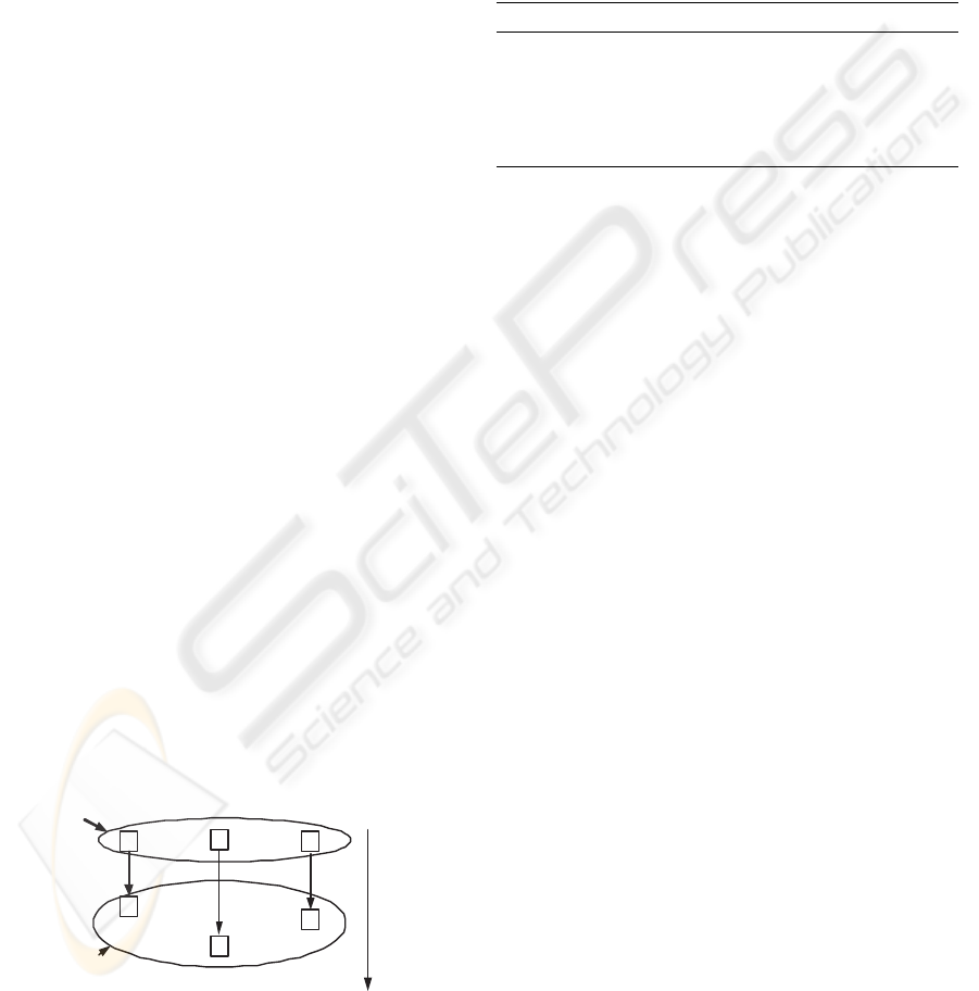
Besides the simple example workflow 1, we have
also simulated a more complicated workflow consist-
ing of 128 tasks as workflow example 2. Workflow
example 2 consists of three loop tasks, 21 split tasks
and 18 merge tasks. Figure 3 shows the makespan
result of all three algorithms on two example work-
flows. Obviously our scheduler has the minimum
makespan, while one-by-one scheduler has the great-
est makespan. As a static approach, one-by-one
scheduler performs the worst in a dynamic grid sce-
nario. The tasks of next level should start after all
tasks of current level have been completed. If there
is a task A requiring much longer execution time than
that of other tasks in current level, there will be a long
period with only one task running since the next level
tasks cannot start until task A finishes. As shown in
Figure 4, our scheduler achieves the lowest cost for
both example workflows; while level-decomposition
algorithm experiences the highest cost. The result is
not surprising since only our scheduler has consid-
ered the cost in scheduling. Furthermore, the longer
the time of their tasks occupying resources, the more
the users should pay.
GRID WORKFLOW SCHEDULING WITH TEMPORAL DECOMPOSITION
445
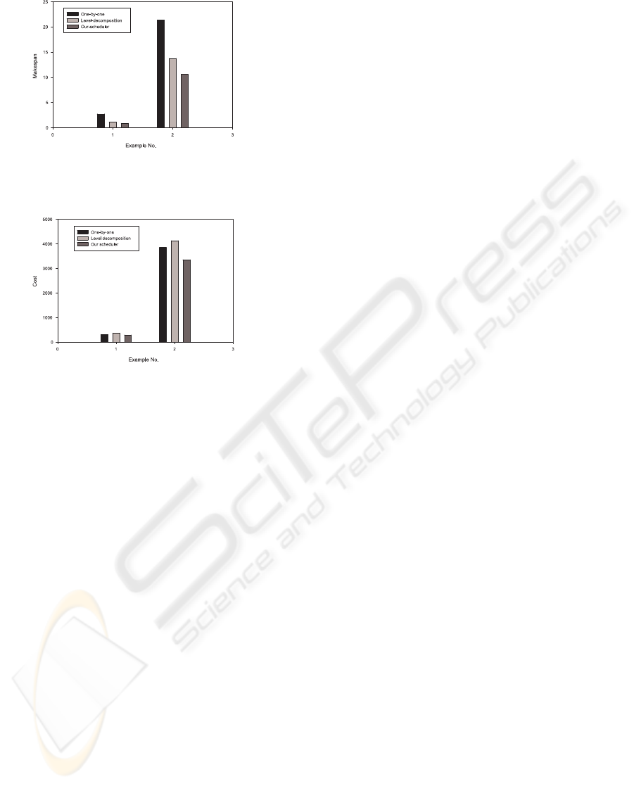
Figure 3: Makespan of example flows.
Figure 4: Cost of example flows.
6 CONCLUSION
In this paper, we propose a “temporal decompo-
sition” scheme to decouple the whole large work-
flow scheduling problem to sub-workflow schedul-
ing problem. An added advantage of our scheme is
its adaptability to dynamic grid resources. The sub-
workflow schedule is chosen according to the latest
states of grid resources, instead of the states at the
start time of workflow. We have also developed an
scheduling algorithm to solve sub-workflow schedul-
ing problem with resource constraints. The prelim-
inary numerical results demonstrate that our scheme
outperforms “one-by-one” and simple “level decom-
position” schemes in both makespan and system cost.
The performance of our scheduler in the presence of
grid resource failures is interesting and will be inves-
tigated in our further work.
REFERENCES
Cardoso, J., Miller, J., Sheth, A., and Arnold, J. (2004).
Modeling quality of service for workflows and web
service processes. Web Semantics Journal: Sci-
ence, Services and Agents on the World Wide Web,
1(3):281–308.
Cheng, J. Q. and Wellman, M. P. (1998). The WALRAS al-
gorithm: A convergent distributed implementation of
general equilibrium outcomes. Computational Eco-
nomics, 12:1–24.
Deelman, E., Blythe, J., Gil, Y., and Carl Kesselman, e.
(2004). Pegasus: Mapping scientific workflows onto
the grid. In AxGrids 2004, LNCS, volume 3165, pages
11–20. Springer Berlin / Heidelberg.
Smale, S. (1976). Convergent process of price adjustment
and global newton methods. American Economic Re-
view, 66(2):284–294.
Wolski, R., Plank, J. S., Brevik, J., and Bryan., T. (2001).
Gcommerce: Market formulations controlling re-
source allocation on the computational grid. In IPDPS
’01: Proceedings of the 15th International Parallel &
Distributed Processing Symposium, page 46, Wash-
ington DC. IEEE Computer Society.
Yu, J. and Buyya, R. (2005). A taxonomy of workflow man-
agement systems for grid computing. Journal of Grid
Computing, 3(3-4):171–200.
Yu, J., Buyya, R., and Tham, C. K. (2005). QoS-
based Scheduling of Workflow Applications on Ser-
vice Grids. In Proc. of the 1st IEEE International
Conference on e-Science and Grid Computing, Mel-
bourne, Australia.
Zhang, S., Gu, N., and Li., S. (2004). Grid workflow based
on dynamic modeling and scheduling. In Information
Technology: Coding and Computing, 2004. Proceed-
ings of 2004 International Conference on, volume 2,
pages 35–39.
ICEIS 2007 - International Conference on Enterprise Information Systems
446
