LEARNING TO RANK FOR COLLABORATIVE FILTERING

Jean-Francois Pessiot, Tuong-Vinh Truong, Nicolas Usunier, Massih-Reza Amini and Patrick Gallinari

Department of Computer Science, University of Paris VI

104 Avenue du President Kennedy, 75016 Paris, France

Keywords:

Collaborative Filtering, Recommender Systems, Machine Learning, Ranking.

Abstract:

Up to now, most contributions to collaborative ﬁltering rely on rating prediction to generate the recommenda-

tions. We, instead, try to correctly rank the items according to the users’ tastes. First, we deﬁne a ranking error

function which takes available pairwise preferences between items into account. Then we design an effec-

tive algorithm that optimizes this error. F inally we illustrate the proposal on a standard collaborative ﬁltering

dataset. We adapted the evaluation protocol proposed by (Marlin, 2004) for rating prediction based systems

to our case, where pairwise preferences are predicted instead. The preliminary results are between those of

two reference rating prediction based methods. We suggest different directions to further explore our ranking

based approach for collaborative ﬁltering.

1 INTRODUCTION

With the emergence of e-commerce, a growing num-

ber of commercial websites are using recommender

systems to help their customers ﬁnd products to pur-

chase. The goal of such systems is to generate person-

alized recommendations for each user, i.e. to ﬁlter out

a potentially huge set of items, and to extract a sub-

set of N items that best matches his tastes or needs.

The most successful approach to date is called collab-

orative ﬁltering; the main underlying idea is to iden-

tify users with similar tastes and use them to generate

the recommendations. Collaborative ﬁltering is par-

ticularly suited to recommend cultural products like

movies, books and music, and is extensively used in

many online commercial recommender systems, like

Amazon.com or CDNow.com.

A simple way to model a user’s preferences is to

assign to each item a numerical score which measures

how much he likes this item. All items are then or-

dered according to those scores, from the user’s top

favorites to the ones he’s less interested in. In the stan-

dard collaborative ﬁltering framework, those scores

are ordinal ratings from 1 to 5. Each user has only

rated a few items, leaving the majority of them un-

rated. Most collaborative ﬁltering methods are based

on a rating prediction approach: taking the available

ratings as input, their goal is to predict the missing

ratings. The recommendation task simply consists in

recommending each user the unrated items with the

highest predictions.

Due to its simplicity and the fact that it easily ac-

commodates with objective performance evaluation,

the rating prediction approach is the most studied in

the collaborative ﬁltering literature. Previous works

include classiﬁcation (Breese et al., 1998), regres-

sion (Herlocker et al., 1999), clustering (Chee et al.,

2001), dimensionality reduction ((Canny, 2002), (Sre-

bro and Jaakkola, 2003)) and probabilistic methods

((Hofmann, 2004), (Marlin, 2003)). As they all re-

duce the recommendation task to a rating prediction

problem, those methods share a common objective:

predicting the missing ratings as accurately as possi-

ble. However, from the recommendation perspective,

the order over the items is more important than their

ratings. Our work is therefore a ranking prediction

approach: rather than trying to predict the missing

ratings, we predict scores that respect pairwise prefer-

ences between items, i.e. preferences expressing that

one item is preferred to another. Using those pairwise

preferences, our goal is to improve the quality of the

recommendation process.

145

Pessiot J., Truong T., Usunier N., Amini M. and Gallinari P. (2007).

LEARNING TO RANK FOR COLLABORATIVE FILTERING.

In Proceedings of the Ninth International Conference on Enterprise Information Systems - AIDSS, pages 145-151

DOI: 10.5220/0002396301450151

 SciTePress

The rest of the paper is organized as follows. Sec-

tion 2 presents our approach, then details the algo-

rithm and the implementation. Experimental protocol

and results are given in section 3. We conclude and

give some suggestions to improve our model in sec-

tion 4.

2 CF AS A RANKING TASK

2.1 Motivation

Most previous works in the collaborative ﬁltering lit-

erature have a common approach where they decom-

pose the recommendation task into two steps: rat-

ing prediction and recommendation. Of course, once

the ratings are predicted, the latter is trivially accom-

plished by sorting the items according to their pre-

dictions and recommending to each user the items

with the highest predictions. As they reduce the rec-

ommendation task to a rating prediction problem, all

these rating prediction approaches have the same ob-

jective: predicting the missing ratings as accurately

as possible. Such objective seems natural for the rec-

ommendation task, and it has been the subject of a

great amount of research in the collaborative ﬁlter-

ing domain (Marlin, 2004). The rating based formu-

lation is simple and easily accommodates with later

performance evaluation. However, it is important to

note that rating prediction is only an intermediate step

toward recommendation, and that other alternatives

may be considered.

In particular, considering the typical use of rec-

ommendation where each user is shown the top-N

items without their predicted scores (Deshpande and

Karypis, 2004), we think that correctly sorting the

items is more important than correctly predicting their

ratings. Although these two objectives look similar,

they are not equivalent from the recommendation per-

spective. Any method which correctly predicts all the

ratings will also correctly sort all the items. However,

two methods equally good at predicting the ratings

may perform differently at predicting the rankings.

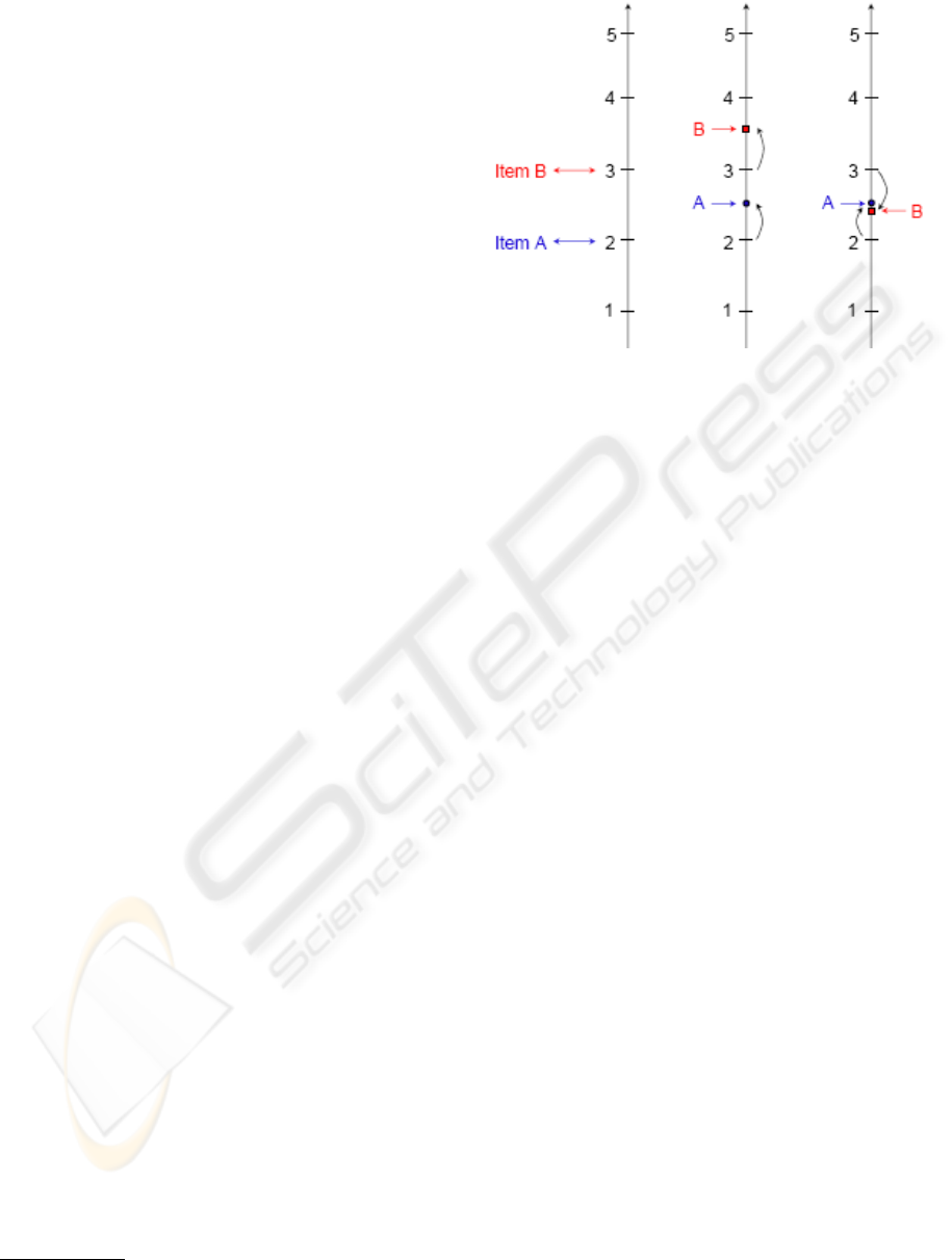
Figure 1 shows a simple example: let [2, 3] be the true

ratings of items A and B respectively, r

= [2.5, 3.6]

and r

= [2.5, 2.4] be two prediction vectors obtained

from two different methods. r

and r

are equivalent

with respect to the squared error

(both errors equal

0.5

+ 0.6

), while only r

predicts the correct rank-

ings, as it scores B higher than A. A more detailed

study of the performance evaluation problem in col-

That is the squared difference between a true rating and

the prediction

Figure 1: Left scale: true ratings for items A and B. Middle

and right scales: prediction vectors r

and r

. The squared

error equals 0.61 for both r

and r

. The ranking error

equals 0 for r1 and 1 for r2.

laborative ﬁltering can be found in (Herlocker et al.,

2004).

This work proposes an alternative to the tradi-

tional rating prediction approach: our goal is to cor-

rectly rank the items rather than to correctly predict

their ratings. To achieve this goal, we ﬁrst deﬁne

a ranking error that penalizes wrong ranking predic-

tions between two items. Then we propose our model,

and design an effective algorithm to minimize the

ranking error.

2.2 Formal Deﬁnition and Notation

2.2.1 Deﬁnition

We assume that there are a set of n users and p items,

and that each user has rated at least one item. A

CF training instance is a triplet of the form (x, a, r)

where x, a and r are respectively a user index in X =

{1, . . . , n}, an item index in Y = {1, . . . , p} and a rat-

ing value in V = {1, . . . , v}. For each user’s available

ratings, we construct the set of pairwise preferences

= {(a, b)|a ∈ Y , b ∈ Y , r

(a) > r

(b)}, where r

(a)

denotes the rating of item a provided by user x. Every

pair (a, b) ∈ y

is called a pairwise preference which

means that user x prefers item a to item b.

2.2.2 Utility Functions

Utility functions are the most natural way to repre-

sent preferences. An utility function f : X × Y → R

depicts the user preferences over a given item as a

real-valued variable. Thus, if an user x ∈ X prefers

ICEIS 2007 - International Conference on Enterprise Information Systems

146

an item a over an item b, this preference can sim-

ply be represented by the inequality f (x, a) > f (x, b).

To make recommendations for a given user x, it then

comes natural to present items in a decreasing order

of ranks with respect to the output of f (x, .).

We consider that each user and each item is de-

scribed by an (unknown) k-length vector, where k is a

ﬁxed integer. We also consider that the form of a util-

ity function f is a dot product between the user vector

and the item vector ∀(x, a) ∈ X ×Y , f (x, a) =

, u

where i

∈ R

and u

∈ R

are respectively the vector

descriptions of item a and user x. We deﬁne U as the

n-by-k matrix where the x-th row contains the user

vector u

, and I as the k-by-p matrix where the a-th

column contains the item vector i

. The product UI

denominates a n-by-p utility matrix associated to the

utility function f , where (U I)

= f (x, a).

2.2.3 Cost Function

With respect to the previous notations, a ranking pre-

diction is correct if f (x, a) > f (x, b) when (a, b) ∈ y

We can now deﬁne the cost function D as the number

of pairwise preferences (a,b) ∈ y

wrongly predicted

by the utility function over all users in the training set:

D(U, I) =

∑

(a,b)∈y

[[(UI)

≤ (UI)

]] (1)

where [[pr]] is equal to 1 if the predicate pr holds and

0 otherwise. The objective of learning is to ﬁnd the

best representations for users and items such that the

number of pairwise preferences wrongly predicted, D,

is the lowest possible. This is an optimisation prob-

lem which consists to ﬁnd I and U minimizing D. As

D is not differentiable we optimise its exponential up-

perbound using the inequality [[x ≤ 0]] ≤ e

−x

D(U, I) ≤

∑

(a,b)∈y

(U I)

−(U I)

{z }

E(U,I)

(2)

The exponential upper-bound is convex separately

in U and I, so standard optimisation algorithms can

be applied for its minimisation. In order to regularize

the factorization, we also add two penalty terms to the

exponential objective function E

R (U, I) =

∑

(a,b)∈y

(U I)

−(U I)

+ µ

kUk

+ µ

kIk

(3)

where kRk

denotes the Frobenius norm of a matrix

R, and is computed as the sum of its squared elements

: kRk

∑

i j

. It is a standard penalty function

used to regularize matrix factorization problems (Sre-

bro et al., 2004). The regularization is controled by

the positive coefﬁcients µ

, µ

and must be carefully

chosen to avoid overﬁtting the model on the training

data. The optimization problem reduces to :

∗

, I

∗

) = argmin

U,I

R (U, I)

where argmin returns the matrices U

∗

and I

∗

that min-

imize the cost function R .

2.3 Model

2.3.1 Optimization

The objective function R is convex over each variable

U and I separately, it is however not convex over both

variables simultaneously. To minimize R , we pro-

pose a two steps optimization procedure, which con-

sists in alternatively ﬁxing one variable U or I and

minimizing R with respect to the other. Each min-

imization step is performed using gradient descent,

and those steps are repeated until convergence. Al-

gorithm 1 depicts this procedure.

Algorithm 1: A learning Algorithm for CF.

Input :

• The set of pairwise preferences

∀x ∈ X , y

= {(a, b)|a ∈ Y , b ∈ Y , r

(a) > r

(b)}

Initialize:

• Initialize U

(1)

and I

(1)

at random

• t ← 1

repeat

• U

(t+1)

← argmin

(t )

R (U

(t)

, I

(t)

)

• I

(t+1)

← argmin

(t )

R (U

(t+1)

, I

(t)

)

• t ← t + 1

until convergence of R (U, I) ;

Output : U and I

As the objective function R is not convex in both U

and I, the proposed algorithm may lead to a local min-

ima of R . The derivatives of R computed at each step

of the algorithm for the gradient descent are:

∂R

∂I

∑

)

−(I

)

−

∑

)

−(I

)

b j

+ 2µ

∂R

∂U

∑

(a,b)∈y

− i

) e

)

−(I

)

+ 2µ

LEARNING TO RANK FOR COLLABORATIVE FILTERING

147

where u

is the x-th row of U, i

is the a-th column

of I, (I

)

is the j

component of the matrix prod-

uct between I and u

, and δ

= 1 if ( j, a) ∈ y

and 0

otherwise.

2.3.2 Implementation and Complexity Analysis

The most important challenge of CF recommendation

systems is to be able to manage a huge volume of data

in real time. For example, the MovieLens dataset

that we considered in our experiments, is constituted

of 1 million ratings for 6,040 users and 3,706 movies.

As a result CF approaches involve a major constraint

of requiring very high computing resources. The real-

time computing and recommending constraints force

recommendation engines to be scalable in terms of

number of users and items. In order to fulﬁll these

constraints, our system learn the parameters U

∗

and

∗

ofﬂine and makes recommendations online. In the

following, we present the computational complexities

of these operations and show that both complexities

are linear in number of items, users or rating’s values.

Ofﬂine Learning Complexity. Learning the pa-

rameters of the recommendation system goes over the

computation of the gradient of R (equation 3) with

respect to U and I (algorithm 1). This computation re-

quires to consider the p

pairwise preferences over all

items and is often unrealistic in real-life CF applica-

tions. However, similarly to (Amini et al., 2005), we

can show that the objective function R can be rewrit-

ten as follows :

R (U, I) =

∑

r∈V

∑

a|r

(a)<r

(U I)

∑

b|r

(b)=r

−(U I)

+ µ

kUk

+ µ

kIk

for which the computation is linear with respect to the

number of items p. More precisely, the computational

complexity of this function is O(np(v + k)) (where

n is the number of users, v the number of possible

rating values and k the dimension of the space rep-

resentation). Using a similar decomposition for both

gradients, the complexity of each iteration of our al-

gorithm is O(np(v + k)). The total complexity is then

O(T np(v + k)), where T is the maximum number of

iterations of our algorithm.

Recommendation Complexity. To make recom-

mendation for a user, the system computes a corre-

sponding score by multiplying the user matrix and

the item matrix. The complexity of this operation

http://www.grouplens.org/

is O(pk), the top h items are then sorted and those

with the highest scores are presented as recommended

items to the user. The complexity of a recommenda-

tion is thus equal to O(p(k + h log h)).

3 EXPERIMENTS

3.1 Experimental Protocol and Error

Measure

In order to evaluate our approach, we are going to

measure the ability of our method to generalize to

unseen pairwise preferences. In these experiments,

the available ratings for each user are split into an

observed set, and a held out set; each set is then

used to generate a pairwise preferences set. The

ﬁrst one is used for training, and the second one for

testing the performance of the method. Note that this

protocol only measures the ability of a method to

generalize to other pairwise preferences provided by

the same users who were used for training the method.

Testing is done by ﬁrst partitioning each user’s

ratings into a set of observed items, and a set of held

out items; each set is then used to generate a pairwise

preferences set: a training one and a test one. One

way to choose the set of held out items is to randomly

pick K items among the user’s ratings. Since CF

datasets are already sparse, for each user we only

pick 2 items for testing and leave the rest for training;

we call this protocol all-but-2.

In order to compare the ranking prediction accuracies

of the different methods, we deﬁne the mean rank-

ing error (MRE), which counts the mean number of

prediction errors over the test pairwise preferences.

Assuming n users and 2 test items per user as in the

all-but-2 protocol:

MRE =

∑

[[(I

)

≤ (I

)

]]

where (a

, b

) is the test pairwise preference of user i.

3.2 Dimensionality Reduction for

Rating Prediction

We compare our approach with two dimensional-

ity reduction methods used for rating prediction:

weighted Singular Value Decomposition and General-

ized Non-Negative Matrix Factorization. In this sub-

section, we brieﬂy describe them and explain how

they are applied to the rating prediction task.

ICEIS 2007 - International Conference on Enterprise Information Systems

148

Deﬁnitions. In the following, R is a n-by-p matrix,

k is a positive integer with k < np, and W is a n-by-p

matrix of positive weights. The Frobenius norm

of R is deﬁned as: kRk

∑

i j

. In its simplest

form, the goal of matrix factorization is to ﬁnd the

best k -rank approximation of R in respect to the

Frobenius norm, i.e. to ﬁnd the k-rank matrix

minimizing kR −

. As most standard matrix

factorization methods are unable to handle missing

elements in R, recent approaches propose to optimize

the weighted Frobenius norm instead of the standard

Frobenius norm, i.e.: kW (R −

R)k

, where  is the

elementwise Schur product. Missing elements R

i j

are

simply handled by setting corresponding W

i j

to 0.

Singular Value Decomposition. SVD is a standard

method for dimensionality reduction; it is used to

decompose R into a product ASV

where A, S, V

are n-by-p, p-by-p, p-by-p matrices respectively. In

addition, A and V are orthogonal, and S is a diagonal

matrix where S

is the i

largest eigenvalue of DD

;

the columns of A and V are the eigenvectors DD

and D

D respectively, and are ordered according to

the values of the corresponding eigenvalues. The

main property is that the k-rank approximation of

R obtained with SVD is optimal in respect to the

Frobenius norm. While SVD cannot be used when

some entries of the target matrix R are missing,

the weighted SVD (wSVD) approach proposed by

(Srebro and Jaakkola, 2003) can handle such missing

data by optimizing the weighted Frobenius norm.

Its simplest implementation consists of an EM-like

algorithm, where SVD is iteratively applied to an

updated low-rank approximation of R. Although very

simple to implement, this method suffers from a high

algorithmic complexity ( O(lnp

+ l p

) where l is

the number of iterations), making it difﬁcult to use on

real CF datasets.

Non-negative Matrix Factorization. NMF is a

matrix factorization method proposed by (Lee and Se-

ung, 1999). Given a non-negative n-by-p matrix R

(i.e. all the elements of R are non-negative real num-

bers), NMF computes a k-rank decomposition of R

under non-negativity constraints. The motivation of

NMF lies in those constraints, as their authors ar-

gue that they allow the decomposition of an object

as the sum of its parts. Formally, we seek a prod-

uct of two non-negative matrices U , I of sizes n-

by-k and k -by-p respectively, optimal in respect to

the Frobenius norm. The corresponding optimiza-

tion problem is not convex, thus only local minima

are achievable; those can be found using Lee’s multi-

plicative updates. Although NMF was not designed to

work with missing data, (Dhillon and Sra, 2006) re-

cently proposed the Generalized Non-negative Matrix

Factorization (GNMF) which optimizes the weighted

Frobenius norm.

Application to CF. . Previous matrix factorization

methods are applied in a similar way to the CF task:

given n users and p items, we consider the n-by-p tar-

get matrix R and the n-by-p weights matrix W . If

the user x provided the rating r for the item a, then

= r and W

= 1; if the rating is unknown, then

i j

= 0. The matrix factorization of R is driven by

the optimization of the weighted Frobenius norm; for

both weighted SVD and GNMF, unknown ratings are

randomly initialized. The ratings predictions for un-

rated items are given by the k-rank matrix resulting

from the matrix factorization. The real predicted rat-

ings induce a total order over the unrated items; in the

following, we will compare our ranking predictions to

the ones obtained by weighted SVD and GNMF.

3.3 Dataset

We used a public movie rating dataset called Movie-

Lens; it contains 1,000,209 ratings collected from

6,040 users over 3,706 movies. Ratings are on a scale

from 1 to 5. The dataset is 95.5% sparse. For each

user we held out 2 test items using the all-but-2 pro-

tocol, leaving 988,129 ratings for training and 12,080

for testing. This was done 5 times, generating a total

of 10 bases for the evaluation. All the results pre-

sented below are averaged over the generated bases.

3.4 Results

We compared our approach to GNMF and wSVD

for several values of the matrix rank k . We stopped

our algorithm after 50 iterations of our two steps

procedure; GNMF was stopped after 1000 iterations.

We also simpliﬁed the regularization problem by

ﬁxing µ

= µ

for both GNMF and our approach;

several regularization values were tried, and the

presented MRE results correspond to the best ones.

GNMF was used with µ

= µ

= 1, and our ranking

approach with µ

= µ

= 100. The main results are:

GNMF wSVD Ranking

k 9 8 8

MRE 0.2658 0.2770 0.2737

LEARNING TO RANK FOR COLLABORATIVE FILTERING

149

Discussion. The optimal values for k are almost

identical for the three approaches; this is not surpris-

ing for GNMF and wSVD, as they are very similar

methods (their only difference lies in the additional

non-negativity constraints for GNMF). But this is in-

teresting for our ranking approach, and it seems that

explaining the users pairwise preferences is as dif-

ﬁcult as explaining their ratings, as they require the

same number of hidden factors.

Although not equivalent, the ranking error used

for evaluation is closely related to the ranking error

optimized by our approach, while GNMF and wSVD

optimize a squared error measuring how well they

predict the ratings. This is why these primary results

are a bit disappointing, as we would have logically

expected our approach to have the best ranking er-

ror. The good performance of GNMF is not surpris-

ing considering that it already performed well (at least

better than wSVD) with respect to rating prediction

(Pessiot et al., 2006). Concerning wSVD, its ranking

error could be improved by increasing the number of

iterations, but the high algorithmic complexity makes

it difﬁcult to use on real datasets such as MovieLens,

especially when the number of items is high. In our

experiments, we had to stop it after only 20 iterations

due to its extreme slowness. Besides, this wSVD is

also limited by its lack of regularization, which is usu-

ally used to avoid the overﬁtting problem.

Further directions need to be explored to complete

and improve those primary results. The ﬁrst direction

concerns user level normalization: when we minimize

the sum of errors (the sum of squared errors for each

rating in GNMF and wSVD, the sum of ranking errors

for each pairwise preference in our approach), users

who have rated lots of items tend to be associated with

higher errors; thus the learning phase focuses on those

users, while ignoring the others. This problem can be

avoided if we give each user the same importance by

considering normalized errors, i.e. by dividing each

user’s error by the number of his pairwise preferences.

The mean ranking error we deﬁne for evaluation is in

fact a normalized error, as we only consider one test

pairwise preference for each user. This is why we

expect that learning with normalized errors will give

better experimental results.

A second direction we want to explore is a more

careful study of stopping criteria. We stopped GNMF

and our ranking approach after ﬁxed numbers of iter-

ations, which seemed to correspond to empirical con-

vergence. In future experiments, we will rather stop

them when the training errors stop decreasing, which

will allow us a more thorough comparison of the three

methods with respect to the training time.

Another question we need to study concerns the

regularization. It is an important feature of a learn-

ing algorithm as it is used to prevent overﬁtting the

training data, thus avoiding bad predictions on unseen

data. In both GNMF and our ranking approach, µ

and µ

are the regularization terms. Setting µ

= µ

0 means no regularization; and the higher they are, the

more matrix norms are penalized. In our experiments

we ﬁxed µ

= µ

for simplicity. By doing this, we im-

plicitly gave gave equal importance for each variable

of our model. In future works, we will study the exact

inﬂuence of those regularization terms, and how they

should be ﬁxed.

Detailed Results. MRE results for several values of

the rank k:

k 7 8 9 10 11

GNMF 0.2696 0.2688 0.2658 0.2679 0.2684

k 5 6 7 8 9

wSVD 0.2847 0.2862 0.2803 0.2770 0.2786

k 6 7 8 9 10

Ranking 0.2752 0.2744 0.2737 0.2743 0.2753

4 CONCLUSION AND

PERSPECTIVES

The rating prediction approach is still actively used

and studied in collaborative ﬁltering problems. Pro-

posed solutions come from various machine learning

ﬁelds such as classiﬁcation, regression, clustering, di-

mensionality reduction or density estimation. Their

common approach is to decompose the recommen-

dation process into a rating prediction step, and the

recommendation step. But from the recommenda-

tion perspective, we think other alternatives than rat-

ing prediction should be considered. In this paper, we

proposed a new ranking approach for collaborative ﬁl-

tering: instead of predicting the ratings as most meth-

ods do, we predict scores that respect pairwise pref-

erences betweens items, as we think correctly sorting

the items is more important than correctly predicting

their ratings. We proposed a new algorithm for rank-

ing prediction, deﬁned a new evaluation protocol and

compared our approach to two rating prediction ap-

proaches. While the primary results are not as good

as we expected with respect to the mean ranking error,

we are conﬁdent they can be explained and improved

by studying user level normalization, convergence cri-

teria and regularization. We are planning to explore

the relations between collaborative ﬁltering and other

tasks such as text analysis (e.g. text segmentation,

(Caillet et al., 2004) ) and multitask learning (Ando

and Zhang, 2005), in order to extend our work to other

ICEIS 2007 - International Conference on Enterprise Information Systems

150

frameworks such as semi-supervised learning (Amini

and Gallinari, 2003).

ACKNOWLEDGEMENTS

The authors would like to thank Trang Vu for her

helpful comments. This work was supported in part

by the IST Programme of the European Commu-

nity, under the PASCAL Network of Excellence, IST-

2002-506778. This publication only reﬂects the au-

thors view.

REFERENCES

Amini, M.-R. and Gallinari, P. (2003). Semi-supervised

learning with explicit misclassiﬁcation modeling. In

Gottlob, G. and Walsh, T., editors, IJCAI, pages 555–

560. Morgan Kaufmann.

Amini, M.-R., Usunier, N., and Gallinari, P. (2005). Auto-

matic text summarization based on word-clusters and

ranking algorithms. In Proceedings of the 27th Euro-

pean Conference on IR Research, ECIR 2005, San-

tiago de Compostela, Spain, March 21-23, Lecture

Notes in Computer Science, pages 142–156. Springer.

Ando and Zhang (2005). A framework for learning predic-

tive structures from multiple tasks and unlabeled data.

Journal of Machine Learning Research.

Breese, J. S., Heckerman, D., and Kadie, C. (1998). Empir-

ical analysis of predictive algorithms for collaborative

ﬁltering. Proceedings of the Fourteenth Conference

on Uncertainty in Artiﬁcial Intelligence.

Caillet, M., Pessiot, J.-F., Amini, M.-R., and Gallinari, P.

(2004). Unsupervised learning with term clustering

for thematic segmentation of texts. In Proceedings of

the 7th Recherche d’Information Assiste par Ordina-

teur, Avignon, France, pages 648–656. CID.

Canny, J. (2002). Collaborative ﬁltering with privacy via

factor analysis. Proceedings of the 25th annual in-

ternational ACM SIGIR conference on Research and

development in information retrieval.

Chee, S., Han, J., and Wang, K. (2001). Rectree: An ef-

ﬁcient collaborative ﬁltering method. In Data Ware-

housing and Knowledge Discovery.

Deshpande, M. and Karypis, G. (2004). Item-based top-

n recommendation algorithms. ACM Transactions on

Information Systems (TOIS).

Dhillon, I. S. and Sra, S. (2006). Generalized nonnega-

tive matrix approximations with bregman divergences.

NIPS.

Herlocker, J., Konstan, J., and Riedl, J. (1999). An algorith-

mic framework for performing collaborative ﬁltering.

Herlocker, J., Konstan, J., Terveen, L., and Riedl, J. (2004).

Evaluating collaborative ﬁltering recommender sys-

tems. ACM Transactions on Information Systems.

Hofmann, T. (2004). Latent semantic models for collabora-

tive ﬁltering. ACM Trans. Inf. Syst., 22(1):89–115.

Lee, D. D. and Seung, H. S. (1999). Learning the parts of

objects by non-negative matrix factorization. Nature.

Marlin, B. (2003). Modeling user rating proﬁles for col-

laborative ﬁltering. Advances in Neural Information

Processing Systems.

Marlin, B. (2004). Collaborative ﬁltering: A machine learn-

ing perspective.

Pessiot, J.-F., Truong, V., Usunier, N., Amini, M., and

Gallinari, P. (2006). Factorisation en matrices non-

negatives pour le ﬁltrage collaboratif. In 3eme Con-

ference en Recherche d’Information et Applications

(CORIA’06), pages 315–326, Lyon.

Srebro, N. and Jaakkola, T. (2003). Weighted low rank ap-

proximation. In ICML ’03. Proceedings of the 20th

international conference on machine learning.

Srebro, N., Rennie, J. D. M., and Jaakkola, T. S. (2004).

Maximum-margin matrix factorization. In Saul, L. K.,

Weiss, Y., and Bottou, l., editors, Advances in Neural

Information Processing Systems 17. MIT Press, Cam-

bridge, MA.

LEARNING TO RANK FOR COLLABORATIVE FILTERING

151