
A Novel Distance Measure for Interval Data
Jie Ouyang and Ishwar K. Sethi
Intelligent Information Engineering Lab
Department of Computer Science and Engineering
Oakland University
48309 Rochester, MI, USA
Abstract. Interval data is attracting attention from the data analysis community
due to its ability to describe complex concepts. Since clustering is an important
data analysis tool, extending these techniques to interval data is important. Ap-
plying traditional clustering methods on interval data loses information inherited
in this particular data type. This paper proposes a novel dissimilarity measure
which explores the internal structure of intervals in a probabilistic manner based
on domain knowledge. Our experiments show that interval clustering based on
the proposed dissimilarity measure produces meaningful results.
1 Introduction
Interval data is a form of symbolic data[1] in which ranges are used rather than single
values. Table 1 gives a small example of interval data.
Table 1. Sample Interval Data.
Age Height Weight Salary
[20,30] [160,170] [80,90] [23000,30000]
[40,50] [150,160] [50,60] [40000,50000]
Interval data can be obtained from rich sources such as the summaries of huge
amounts of numerical data, the answers to questionnaires, and instances where the val-
ues of the observations are uncertain by nature. Data analysis of interval data gets atten-
tion due to its rich sources and ability to describe complex concepts. Interval patterns
are described by features which are ranges over real axis. Formally, a p dimensional
interval pattern X can be expressed as X = ([x
−
1
, x
+
2
], ..., [x
−
p
, x
+
p
]), where x
−
i
and
x
+
i
are the lower and upper bounds of the ith feature of X respectively. Interval data
conveys more information than numerical data. A numerical data usually represents the
distance from the origin in its coordinate system while a interval provides at least two
types of information: the location and the length of that interval. The length or span of
an interval is also called internal structure.
Ouyang J. and K. Sethi I. (2007).
A Novel Distance Measure for Interval Data.
In Proceedings of the 7th International Workshop on Pattern Recognition in Information Systems, pages 49-58
DOI: 10.5220/0002425000490058
Copyright
c
SciTePress

Clustering is a powerful data analysis tool. Data clustering aims to partition a set
of patterns into groups such that similar patterns are grouped together. Clustering of
numerical data has drawn intensive research over the last several decades. Comprehen-
sive review literatures can be found in [2] and [3]. Interval clustering solves the same
problem as traditional clustering except the objects to be clustered are interval data. Dis-
similarity measures and optimization algorithms are two key components of the clus-
tering methods. Applying traditional distance measures on prototypes of intervals, such
as means or medians, loses information on the internal structure. Hence dissimilarity
estimation for interval data is a new challenge and also the subject of this work.
Section 2 reviews distance measures and optimization methods used in some related
work on interval clustering. Section 3 introduces our distance measure based on proba-
bility density functions(pdfs). We show some promising experimental results based on
the new dissimilarity in section 4, and a short conclusion is given in the last section.
In terms of notation, capital letters are used for patterns and small letters are used for
features or singleton patterns.
2 Related work
This section reviews some previous work on interval clustering with a focus on distance
measures and optimization methods. When talking about distance measures, we denote
distance between two patterns by D
X,Y
and distance between two features by d
X
i
,Y
i
.
The Hausdorff distance metric is widely used for interval data. Carvalho et al.[4]
proposed a dynamic interval clustering method based on Hausdorff distance. The dis-
tance between pattern X and a prototype, Y
k
, of cluster C
k
is defined as D
X,Y
k
=
P
p
i=1
λ
k,i
d
X
i
,Y
k,i
, where d
X
i
,Y
k,i
is the Hausdorff distance defined as max(|x
−
i
−
Y
−
k,i
|, |x
+
i
− Y
+
k,i
|). The interesting point is that each cluster is associated with a p di-
mensional weight vector λ. The optimization method consists of three steps. The first
step tries to find the cluster prototypes Y
k
s such that
P
X∈C
k
d
X
i
,Y
k,i
is minimized for
each feature i. The second step happens after the Y
k
is determined. It seeks to find the
λ
k
such that the
P
X∈C
k
D
X,Y
k
is minimized. The third step reallocates patterns. The
relocation of patterns and optimization steps are repeated until no patterns need to be
relocated. Souze and Carvalho applied the same dynamic clustering framework with
Hausdorff distance replaced by Chebyshev[5] and city block distance[6].
The Hausdorff is also used in [7]. The objects under study are not hyper-boxes
but convex shapes. The dimensions of the original data are first reduced by PCA for
interval data. Six interval PCA methods(V-PCA, C-PCA, S-PCA, RTPCA, LP MR-
PCA and DG MR-PCA) are introduced and the computational problems are addressed.
The projection of original hyper-boxes are convex hulls. The Hausdorff distance is used
to measure dissimilarity of convex hulls and hierarchal clustering is used to classify
them.
Carvalho et al.[8] proposed a partition based interval clustering using L
2
(Minkowski)
distance. L
2
distance is defined as D
X,Y
=
P
p
i=1
d
X
i
,Y
i
, where d
X
i
,Y
i
= |X
−
i
−
Y
−
i
|
2
+ |X
+
i
− Y
+
i
|
2
. A standard optimization step is followed, in which clustering
prototype determination is followed by relocation of patterns. The scaling problem is
addressed in this work. Difference in variable scales results in bias when calculating
50

the distance; L
2
distance measures favor features with big scales and depress the dis-
cernment ability of small scale features. Three standardization methods were proposed,
based on the dispersion of the interval centers, the dispersion of the interval bound-
aries, and the global range. Although these methods normalize the dispersions, they are
sensitive to outliers.
Asharaf et al.[9] proposed an incremental clustering method based on rough set
theory, and using the Minkowski distance measure. Their work emphasizes scalability
and requires only one scan of the data set. The rough set approach naturally handles the
inherent uncertainty of the clustering procedure. Two thresholds are needed; however,
the authors did not explain how to estimate them in real world applications.
Guru and Kiranagi introduced the concept of mutual distance in [10]. Their idea is
that the dissimilarity of X to Y is not necessarily the same as the dissimilarity of Y to
X. Hence d
X
i
→Y
i
and d
Y
i
→X
i
are both defined. The dissimilarity, d
X
i
→Y
i
= (|X
i
| +
[max(X
−
i
, Y
−
i
) − min(X
+
i
, Y
+
i
)])/|Y
i
|. The total dissimilarity takes into account the
length of X
i
, Y
i
and their separability. d
X
i
,Y
i
is the length of the weighted combination
of d
X
i
→Y
i
and d
Y
i
→X
i
such that d
X
i
,Y
i
= |αd
X
i
→Y
i
+ βd
Y
i
→X
i
|. The optimization
method used is hierarchal agglomeration.
Peng and Li[11] summarized dissimilarity measures for interval data. They catego-
rized dissimilarity measures into traditional and modified measures. Traditional meth-
ods only measure distance between the means or median points of the intervals; while
modified methods take into account the boundaries or the structure of the intervals. It is
easy to see the modified methods are more natural than the traditional methods with re-
spect to interval data. They reported empirically that modified distance produces more
accurate clustering results than traditional distance. Also they proposed a two-stage
clustering method. Traditional distance is first used to get a rough structure of clusters,
then the modified distance is then used to generate fine separated clusters. This method
saves unnecessary computation so that the scalability is improved. However it is hard
to decide how many clusters to be generated in the first step when the real number of
clusters is unknown.
3 Proposed Measure of Dissimilarity
3.1 Dissimilarity between Intervals
The dissimilarity, particularly for interval data, should take into consideration the in-
formation of both the position and the span of an interval. As Peng et al. empirically
demonstrated in[11], clustering based on modified distances consistently improved clus-
tering quality. Our dissimilarity has two parts which explicitly compute the dissimilarity
over the span and relative positions respectively.
Given two p dimensional interval patterns X = ([x
−
1
, x
+
2
], ..., [x
−
p
, x
+
p
]) and Y =
([y
−
1
, y
+
2
], ..., [y
−
p
, y
+
p
]), the distance between X and Y is a L
2
distance:
D(X, Y ) =
v
u
u
t
p
X
i=1
d
2
(x
i
, y
i
), (1)
51

where d(x
i
, y
i
) is the distance on feature i. d(x
i
, y
i
) is a weighted combination of two
components in the form:
d(x
i
, y
i
) = α ∗ (1 − s
span) + β ∗ d pos, (2)
where s
span measures similarity over the span and thus 1−s span is the dissimilarity
over the span; d
pos is the dissimilarity over the relative positions; α and β are weight
coefficients and satisfy: α ≥ 0, β ≥ 0 and α + β = 1.
3.2 Dissimilarity Components
When calculating dissimilarity over spans, a family of pdfs is assumed to be associated
with each feature. To simplify the discussion, let f(x|ξ, o, ...) denote the parameterized
pdf of feature x. We argue this assumption is reasonable. In real world application,
each feature has its physical meaning. As mentioned in introduction, interval data is
usually used to summarize huge amount of individual observations or to express certain
degrees of (un)certainty of observations[1]. Hence in practice, we can obtain, from
domain experts or density estimation over individual data, a general pdf for each feature.
In the case that a general pdf cannot be obtained, a general Gaussian distribution, which
is usually reasonable, or a uniform distribution can be assumed.
After deciding the general form of the pdf f (x|ξ, o, ...), the parameters for the pdf
will be determined for each interval of x. These parameters can be estimated by interval
boundaries. The interval stands for the range of the values which have an observed
frequency higher than a certain level, meaning the interval is the support of the assumed
pdf. For example, regarding the jth interval of feature x, we have:
P r(x
−
j
≤ x
j
≤ x
+
j
|ξ, o, ...) =
Z
x
+
j
x
−
j
f(x|ξ, o, ...) ≥ 0.99, (3)
where x
−
j
and x
+
j
are the lower and upper boundaries respectively. The parameters can
be determined by solving Eq. 3. As an example, the parameters of a normal distribution,
with mean µ and standard deviation σ, can easily be obtained from the boundaries a and
b, by letting µ = (a + b)/2 and σ = (b − µ)/3. If only a subset of the parameters is
relevant to the interval spans, all pdfs share the same values of the irrelevant parameters.
In this way all pdfs have the same general shapes. That is, they are all concave or convex
functions. In this case, only a rough approximation of the underlining pdfs is obtained. It
has minor impact on the final results, however, in that i) all intervals of a certain feature
have the same pdf shape and only the supports differ, and ii) our primary interest is the
dissimilarity level not the exact forms of the pdfs.
Once the form of the pdf for a particular interval has been determined, we can
calculate the similarity of the span, s
span of Eq. 2, as the overlapping part of the
aligned pdfs over two intervals:
s
span = pdf′(x|ξ
x
, o
x
, ...)
\
pdf′(y|ξ
y
, o
y
, ...). (4)
Thus s
span depends only on the span of the intervals. To calculate s span, imagine
that the two pdfs are moved together so that the two means overlap. The motivation of
52
calculating 1 − s span is to capture the probabilistic difference of assigning an indi-
vidual observation to different intervals. It is easy to see that 1 − s
span ∈ [0, 1] and
equals 0 when two pdfs have exactly the same shapes. The dissimilarity over relative
position is calculated by the ratio of the spatial difference of means to the total range of
the two intervals. Formally,
d pos =
|mean(x) − mean(y)|
max(x
+
, y
+
) − min(x
−
, y
−
)
. (5)
Also it is easy to see that d
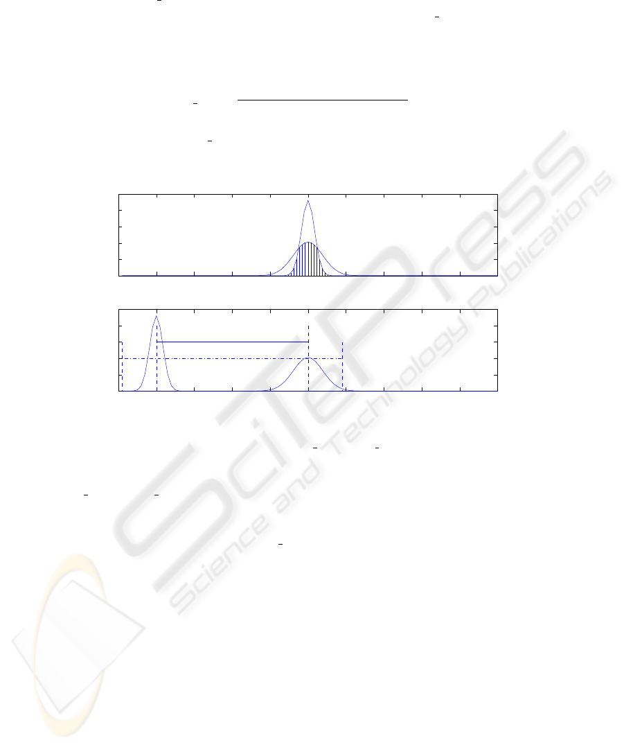
pos ∈ [0, 1]. As an example, Fig. 1. depicts the calculations
0 10 20 30 40 50 60 70 80 90 100
0
0.05
0.1
0.15
0.2
0.25
Distance over interval span
Probability
0 10 20 30 40 50 60 70 80 90 100
0
0.05
0.1
0.15
0.2
0.25
Distance over relative position
Probability
Fig.1. Calculation of s span and d pos.
of s
span and d pos for two interval variables x = ([5, 95]) and y = ([1, 19]). For
simplicity, the estimated pdfs are Gaussian f(x|50, 15) and f(y|10, 3). In the upper
subplot in Fig. 1, pdfs of x and y are moved together as described previously and the
area of the region with vertical bars is s
span. In the lower subplot in Fig. 1, the length
of the solid line is the distance between means and the length of dash-dot line is the
total range of the two intervals.
3.3 Advantages of the Proposed Dissimilarity Measure
Although a few dissimilarity measures proposed in the literature such as modified dis-
tance in[11] take into account the internal structure of interval data, they are heuristic
to some extent. By assuming probability distribution, a probabilistic view of how to uti-
lize the information of interval span can be given. Actually, our approach uses a similar
idea as the Kolmogorov-Smirnov test(KS-test), which can be used to test if two pop-
ulations are from the same underlining probability. Instead of doing hypothesis tests,
we directly use the nonoverlapping part of the pdfs as the dissimilarity caused by the
53

difference in spans. In this way, we use more information about the interval length than
other approaches do. In Eq. 2, the dissimilarity of internal structure has a weight coeffi-
cient α hence it always contributes(if α > 0) to the overall dissimilarity even when two
intervals do not overlap at all.
Our method solves the scaling problem described in[8] in a natural way. The actual
value we consider is the difference of pdfs and since the area under any pdf is 1, every
feature has the same scale.
Additionally, our method is flexible in that domain knowledge can be easily incor-
porated when it is available. On the other hand, a normal or uniform distribution can be
used to approximate the unknown probability distribution if no domain knowledge is
available.
4 Experimental Results
Allocation and hierarchal based clustering methods are the most widely used approaches
in practice. Thus our experiments use complete-linkage based hierarchal clustering. Hi-
erarchal clustering does not require initial user input parameters and is more robust to
the order of patterns than allocation based clustering. Its main drawback, however, is
high computational complexity, which has been improved by some researchers. The fol-
lowing experiments use the same optimization method with different distance measures
and the results are compared. Experiment results are shown for three real world data sets
to demonstrate that clustering methods based on our distance measure can get mean-
ingful results. In the following, we denote our distance measure by P-distance since our
method differs from others by using the probability density function over intervals.
4.1 Fish Data Set
The first experiment is on a fish data set based on 67 fishes whose species and mercury
concentrations in 6 organs have been recorded. The interval data is a summary of indi-
vidual observations. The data set can be obtained at http://www-rocq.inria.
fr/sodas/WP6/data/data.html. The data set consists of 12 patterns according
to 12 fish species which are classified into 4 groups, see Table 2.
In this experiment α and β are set to 0.2 and 0.8 respectively. Because of lack of
domain knowledge, we assume the estimated pdfs for all features are uniform distribu-
tions. Entropy[12] is used to evaluate the clustering quality since the correct classifica-
tion is known. Given a particular cluster S
r
of size n
r
, the entropy of this cluster is
defined to be E(S
r
) =
−1
log q
P
q
i=1
n
i
r
n
r
log
n
i
r
n
r
, where q is the number of classes in the
dataset and n
i
r
is the number of patterns of the ith class that were assigned to the rth
cluster. The entropy of the entire solution is defined to be the sum of the individual clus-
ter entropies weighted according to the cluster size, i.e., Entropy =
P
k
r=1
n
r
n
E(S
r
).
We compare the results obtained by using Hausdorff, modified L
1
, modified L
2
[11]
and P-distance measures. The clustering results and entropy values are shown in Ta-
ble 3. This table shows that the modified L
1
and L
2
measures performed the same,
Hausdorff outperformed these two distances and P-distance performed the best. This
result demonstrates the usefulness of our distance measure. Please note that we are
54

Table 2. Fish Data Set.
Name LONG POID ... Inte/M Esto/M REGIME
Ageneiosusbrevifili [22.5, 35.5] [170, 625] ... [0.23, 0.63] [0, 0.55] 1
Cynodongibbus [19, 32] [77, 359] ... [0, 0.5] [0.2, 1.24] 1
Hopliasaimara [25.5, 63] [340, 5500] ... [0.11, 0.49] [0.09, 0.4] 1
Potamotrygonhystrix [20.5, 45] [400, 6250] ... [0, 1.25] [0, 0.5] 1
Leporinusfasciatus [18.8, 25] [125, 273] ... [0, 0] [0.12, 0.17] 3
Leporinusfrederici [23, 24.5] [290, 350] ... [0.18, 0.24] [0.13, 0.58] 3
Dorasmicropoeus [19.2, 31] [128, 505] ... [0, 1.48] [0, 0.79] 2
Platydorascostatus [13.7, 25] [60, 413] ... [0.3, 1.45] [0, 0.61] 2
Pseudoancistrusbarbatus [13, 20.5] [55, 210] ... [0, 2.31] [0.49, 1.36] 2
Semaprochilodusvari [22, 28] [330, 700] ... [0.4, 1.68] [0, 1.25] 2
Acnodonoligacanthus [10, 16.2] [34.9, 154.7] ... [0, 2.16] [0.23, 5.97] 4
Myleusrubripinis [12.3, 18] [80, 275] ... [0, 0] [0.31, 4.33] 4
Table 3. Clustering result on fish data set.
Distance measures Classification Entropy
P-distance [1 2 3],[5 6],[4 7 8 10],[9 11 12] 0.2500
Hausdorff [1 3],[2],[4 5 6 7 8 10],[9 11 12] 0.4796
Modified L
1
[1 4 5 6 8 9 11 12],[2],[3 7],[10] 0.7500
Modified L
2
[1 4 5 6 8 9 11 12],[2],[3 7],[10] 0.7500
not claiming universal advantage of our approach. Actually the result of our approach
is the same as the results achieved using adaptive L
1
and Hausdorff[4]. However the
approaches in[4] suffer from the common problems of allocation based methods.
4.2 Fat and Oil Data Set
The second data set we used is the Fat and Oil data set[1]. This data set collects 4
features of oil and fat obtained from 6 plants and 2 animals. The data set is shown
in Table 4. For this experiment α and β are set to 0.2 and 0.8 respectively and the
Table 4. Fat and Oil data set.
ID Name GRA FRE IOD SAP
1 Linseed [0.930,0.935] [-27.0,-18.0] [170.0,204.0] [118.0,196.0]
2 Perilla [0.930,0.937] [-5.0,-4.0] [192.0,208.0] [188.0,197.0]
3 Cotton [0.916,0.918] [-6.0,-1.0] [99.0,113.0] [189.0,198.0]
4 Sesame [0.920,0.926] [-6.0,-4.0] [104.0,116.0] [187.0,193.0]
5 Camellia [0.916,0.917] [-21.0,-15.0] [80.0,82.0] [189.0,193.0]
6 Olive [0.914,0.919] [0.0,6.0] [79.0,90.0] [187.0,196.0]
7 Beef [0.860,0.870] [30.0,38.0] [40.0,48.0] [190.0,199.0]
8 Hog [0.858,0.864] [22.0,32.0] [53.0,77.0] [190.0,202.0]
estimated pdfs are normal distributions. As with the previous experiment, clustering
55
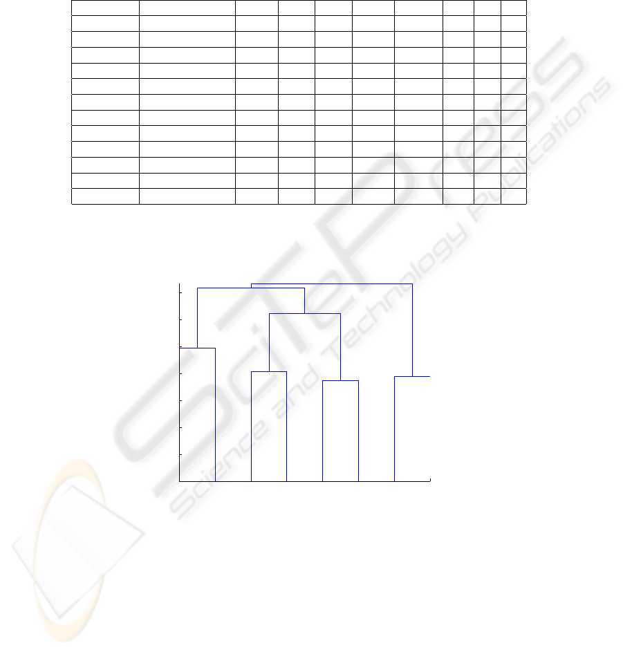
results from different distance measures are compared. The results are compared based
on the background knowledge. The clustering results are shown in Table 5 and the
dendrogram is shown in Fig. 2.
Table 5. Clustering result on fat and oil data set.
# of Clusters Distance measures Linseed Perilla Cotton Sesame Camellia Olive Beef Hog
k=4 P-distance 1 1 2 2 3 3 4 4
k=4 Hausdorff 1 1 2 2 3 3 4 4
k=4 Modified L
1
1 2 3 3 3 3 4 4
k=4 Modified L
2
1 2 3 3 3 3 4 4
k=3 P-distance 1 1 2 2 2 2 3 3
k=3 Hausdorff 1 1 2 2 2 2 3 3
k=3 Modified L
1
1 1 2 2 2 2 3 3
k=3 Modified L
2
1 1 2 2 2 2 3 3
k=2 P-distance 1 1 1 1 1 1 2 2
k=2 Hausdorff 1 1 2 2 2 2 2 2
k=2 Modified L
1
1 1 2 2 2 2 2 2
k=2 Modified L
2
1 1 2 2 2 2 2 2
0
0.2
0.4
0.6
0.8
1
1.2
1.4
Data index
Distance
Dendrogram
1
2
3
4
5
6
7
8
Fig.2. Dendrogram of clustering on Fat and Oil data set.
In this experiment we compare the performance of different distance measures ac-
cording to different number of clusters, denoted by k. The number of clusters is an input
parameter for allocation based methods. However it is usually unknown in practice and
the results are generated in a trial-and-error manner. Hence it is a desired property for
a clustering method to render reasonable results for a range of this parameter. Table 5
56

shows, again, the modified L
1
and L
2
measures performed the same. They correctly
classified patterns only for k = 3. The Hausdorff method performed better than the
modified L
1
and L
2
methods in that it generated the right classification for the cases of
k = 3 and k = 4. These three methods all misclassified patterns when only two clusters
are needed: 4 plant oils are grouped together with fat from animals. Only the results
obtained by using P-distance are robust through the three options of k. When the k is
set to 4, the result is consistent with the fact that linseed and perilla are used for paint,
cotton and sesame are for foods, camellia and olive are for cosmetics[13]. When k is 3,
the result is the same as the one obtained in[1] by Galois lattice. When k is set to 2, the
plant oils are grouped together and separated from the animal fat.
4.3 Temperature Data Set
The last experiment was conducted on the Long-Term Instrumental Climatic Database
of the Peoples Republic of China. This Database contains 900 monthly temperatures
for 12 months observed in 60 meteorological stations of China from 1974 to 1988.
This experiment tests the performance of our method on mid-size data. The correctness
of the clustering results is again measured by entropy. Table 6 shows the entropy of
the clustering using the Hausdorff distance, and the proposed distance with different α
levels.
Table 6. Performance on temperature data set.
α 0.1 0.2 0.3 0.4 0.5 0.6 0.7 0.8 0.9 1
Entropy(P-distance) 0.3152 0.3107 0.3044 0.2920 0.2821 0.2715 0.2594 0.2837 0.3245 0.4231
Entropy(Hausdorff) 0.4561
Our method performs better than Hausdorff for all the α values. The optimal result
is obtained when α = 0.7 which indicates that for certain domains(temperature in this
case), the span may be more important than the position of the intervals when measuring
(dis)similarities.
4.4 Discussion
From the above experimental results we can see that our approach gets better results
than other methods in some situations. However our method has three parameters to
be tuned. The underlining density function over each interval can be obtained from
domain knowledge or simply assumed to be gaussian or uniform. The idea of providing
α and β is to give users a chance to weight the dissimilarities over span and location.
However the performance of our distance measure depends on the choices of α and β.
The values of these two parameters were obtained by a trial-and-error manner in our
experiments. The stability of clustering algorithms against α and β is also tested(only
observations are reported here due to space limitations). The optimal results in Table 2
for the fish data set can be obtained over a wide range of α, which is from 0.2 to 1. The
57

optimal results in Table 4 for fat and oil data set can be obtained over a small range of
α, which is from 0.1 to 0.2, and one pattern is misclassified for the case that k = 4 and
0.3 ≤ α ≤ 0.7. How to improve the robustness of the clustering algorithm with respect
to the parameters and how to automatically determine the values of α and β can be the
topics of future work.
5 Conclusion
In this work, we presented a novel dissimilarity measure for interval data. This dissim-
ilarity provides a framework to incorporate domain knowledge. Also it gives a proba-
bilistic view of exploring the dissimilarity(similarity) over the interval’s internal struc-
ture. Experiments on clustering algorithms based on the new dissimilarity were con-
ducted with promising results. Future work may include improving the robustness and
automatically determining the parameter settings.
References
1. Hans Hermann Bock: Analysis of Symbolic Data: Exploratory Methods for Extracting Sta-
tistical Information from Complex Data. Springer-Verlag New York, Inc. Secaucus, NJ, USA
(2000)
2. A. K. Jain, M. N. Murty, P. J. Flynn: Data clustering: A Review. ACM Computing Surveys
Vol. 31 No. 3 (1999) 264-323
3. Rui Xu, Donald Wunsch II: Survey of Clustering Algorithms. IEEE Transactions on Neural
Networks Vol. 16 No. 3 (2005) 645–678
4. Francisco de A. T. de Carvalho, Renata M. C. R. de Souza, Marie Chavent, Yves Lecheval-
lier: Adaptive Hausdorff Distances and Dynamic Clustering of Symbolic Interval Data. Pat-
tern Recognition Letters Vol. 27 No. 3 (2006) 167–179
5. R.M.C.R. de Souza, F.A.T. de Carvalho: Dynamic Clustering of Interval Data Based on
Adaptive Chebyshev Distances. Electronics Letters Vol. 40 No. 11 (2004) 658–660
6. Renata M. C. R. de Souza, Francisco de A. T. de Carvalho: Clustering of Interval Data Based
on City-block Distances. Pattern Recognition Letters Vol. 25 No. 3 (2004) 353–365
7. Antonio Irpino, Valentino Tontodonato: Clustering Reduced Interval Data Using Hausdorff
Distance. Computational Statistics Vol. 21 No. 2 (2006) 271–288
8. Francisco de A. T. de Carvalho, Paula Brito, Hans-Hermann Bock: Dynamic Clustering for
Interval Data Based on L
2
Distance. Computational Statistics Vol. 21 No. 2 (2006) 231–250
9. S. Asharaf, M. Narasimha Murty, S. K. Shevade: Rough Set Based Incremental Clustering
of Interval Data. Pattern Recognition Letters Vol. 27 No. 6 (2006) 515–519
10. D.S. Guru, Bapu B. Kiranagi: Multivalued Type Dissimilarity Measure and Concept of Mu-
tual Dissimilarity Value for Clustering Symbolic Patterns. Pattern Recognition Vol. 38 No. 1
(2005) 151–156
11. Wei Peng, Tao Li: Interval Data Clustering with Applications. Tools with Artificial Intelli-
gence, 18th IEEE International Conference on (2006) 355–362
12. Ying Zhao, George Karypis: Empirical and Theoretical Comparisons of Selected Criterion
Functions for Document Clustering. Machine Learning Vol. 55 No. 3 (2004) 311–331
13. Manabu Ichino, Hiroyuki Yaguchi: Generalized Minkowski Metrics for Mixed Fature-type
Data Analysis. IEEE Transactions on Systems, Man, and Cybernetics Vol. 24 No. 4 (1994)
698–708
58
