
Bridging the Gap between Naive Bayes and Maximum
Entropy Text Classification
⋆
Alfons Juan
1
, David Vilar
2
and Hermann Ney
2
1
DSIC/ITI, Univ. Polit
`
ecnica de Val
`
encia, E-46022 Val
`
encia, Spain
2
Lehrstuhl f
¨
ur Informatik 6, RWTH Aachen, D-52056 Aachen, Germany
Abstract. The naive Bayes and maximum entropy approaches to text classifi-
cation are typically discussed as completely unrelated techniques. In this paper,
however, we show that both approaches are simply two different ways of doing
parameter estimation for a common log-linear model of class posteriors. In par-
ticular, we show how to map the solution given by maximum entropy into an
optimal solution for naive Bayes according to the conditional maximum likeli-
hood criterion.
1 Introduction
The naive Bayes and maximum entropy text classifiers are well-known techniques for
text classification [1, 2]. Both techniques work with text documents represented as word
counts. Also, both are log-linear decision rules in which an independent parameter is
assigned to each class-word pair so as to measure their relative degree of association.
Apparently, the only significant difference between them is the training criterion used
for parameter estimation: conventional (joint) maximum likelihood for naive Bayes and
conditional maximum likelihood for (the dual problem of) maximum entropy [2, 3].
This notable similarity, however, seems to have passed unnoticed for most researchers
in text classification and, in fact, naive Bayes and maximum entropy are still discussed
as unrelated methods.
In this paper, we provide a direct, bidirectional link between the naive Bayes and
maximum entropy models for class posteriors. Using this link, maximum entropy can
be interpreted as a way to train the naive Bayes model with conditional maximum likeli-
hood. This is shown in Section 3, after a brief review of naive Bayes in the next section.
Empirical results are reported in Section 4, and some concluding remarks are given in
Section 5.
2 Naive Bayes Model
We denote the class variable by c = 1, . . . , C, the word variable by d = 1, . . . , D, and
a document of length L by d
L
1
= d
1
d
2
· · · d
L
. The joint probability of occurrence of c,
⋆
Work supported by the EC (FEDER) and the Spanish “Ministerio de Educaci
´
on y Ciencia”
under grants TIN2006-15694-CO2-01 (iTransDoc research project) and PR-2005-0196 (fel-
lowship from the “Secretar
´
ıa de Estado de Universidades e Investigaci
´
on”).
Juan A., Vilar D. and Ney H. (2007).
Bridging the Gap between Naive Bayes and Maximum Entropy Text Classification.
In Proceedings of the 7th International Workshop on Pattern Recognition in Information Systems, pages 59-65
DOI: 10.5220/0002425700590065
Copyright
c
SciTePress

L and d
L
1
may be written as:
p(c, L, d
L
1
) = p(c) p(L) p(d
L
1
| c, L) (1)
where we have assumed that document length does not depend on the class.
Given the class c and the document length L, the probability of occurrence of any
particular document d
L
1
can be greatly simplified by making the so-called naive Bayes
or independence assumption: the probability of occurrence of a word d
l
in d
L
1
does not
depend on its position l or other words d
l
′
, l
′
6= l ,
p(d
L
1
| c, L) =
L
Q
i=1
p(d
i
| c) (2)
Using the above assumptions, we may write the posterior probability of a document
belonging to a class c as:
p(c | L, d
L
1
) =
p(c, L, d
L
1
)
P
c
′
p(c
′
, L, d
L
1
)
(3)
=
ϑ(c)
Q
D
d=1
ϑ(d | c)
x
d
P
c
′
ϑ(c
′
)
Q
D
d=1
ϑ(d | c
′
)
x
d
(4)
△
= p
θ
(c | x) (5)
where x
d
is the count of word d in d
L
1
, x = (x
1
, . . . , x
D
)
t
, and θ is the set of unknown
parameters, which includes ϑ(c) for the class c prior and ϑ(d | c) for the probability
of occurrence of word d in a document from class c. Clearly, these parameters must be
non-negative and satisfy the normalisation constraints:
P
c
ϑ(c) = 1 (6)
P
D
d=1
ϑ(d | c) = 1 (c = 1, . . . , C) (7)
The Bayes’ decision rule associated with model (5) is a log-linear classifier:
x → c
θ
(x) = arg max
c
p
θ
(c | x) (8)
= arg max
c
(
log ϑ(c) +
X
d
x
d
log ϑ(d | c)
)
(9)
3 Naive Bayes Training and Maximum Entropy
Naive Bayes training refers to the problem of deciding (a criterion and) a method to
compute an appropriate estimate for θ from a given collection of N labelled training
samples (x
1
, c
1
), . . . , (x
N
, c
N
). A standard training criterion is the joint log-likelihood
function:
L(θ) =
P
n
log p
θ
(x
n
, c
n
) (10)
=
P
c
N
c
log ϑ(c) +
P
d
N
cd
log ϑ(d | c) (11)
60

where N
c
is the number of documents in class c and N
cd
is the number of occurrences
of word d in training data from class c. It is well-known that the global maximum of (10)
under constraints (6)-(7) can be computed in closed-form:
ˆ
ϑ(c) =
N
c
N
(12)
and
ˆ
ϑ(d | c) =
N
cd
P
d
′
N
cd
′
(13)
This computation is usually preceded by a preprocessing step in which documents are
normalised in length so as to avoid parameter estimates being excessively influenced by
long documents [4]. After training, this preprocessing step is no longer needed since the
decision rule (8) is invariant to length normalisation. In what follows, we will assume
that documents are normalised to unit length, i.e.
P
d
x
d
= 1.
In this paper, we are interested in the conditional log-likelihood criterion:
CL(θ) =
X
n
log p
θ
(c
n
| x
n
) (14)
which is to be maximised under constraints (6)-(7). To this end, consider the conven-
tional maximum entropy text classification model, as defined in [2]:
p
Λ
(c | x) =
exp
P
i
λ
i
f
i
(x, c)
P
c
′
exp
P
i
λ
i
f
i
(x, c
′
)
(15)
where the set Λ = {λ
i
} includes, for each class-word pair i = (c
′
, d
′
), a (free) parame-
ter λ
i
∈ IR for its associated feature:
f
i
(x, c) = f
c
′
d
′
(x, c) =
(
x
d
′
if c
′
= c
0 otherwise
(16)
61

Given an arbitrary value of the lambdas,
˜
Λ = {
˜
λ
i
}, we have:
p
˜
Λ
(c|x)=
exp
P
d
˜
λ
cd
x
d
P
c
′
exp
P
d
˜
λ
c
′
d
x
d
(17)
=
Q
d
˜α
x
d
cd
P
c
′
Q
d
˜α
x
d
c
′
d
with: ˜α
cd
△
= exp(
˜
λ
cd
) (18)
=
Q
d
˜
ϑ(c, d)
x
d
P
c
′
Q
d
˜
ϑ(c
′
, d)
x
d
˜
ϑ(c, d)
△
=
˜α
cd
P
c
′
P
d
′
˜α
c
′
d
′
(19)
=
˜
ϑ(c)
Q
d
h
˜
ϑ(c,d)
˜
ϑ(c)
i
x
d
P
c
′
˜
ϑ(c
′
)
Q
d
h
˜
ϑ(c
′
,d)
˜
ϑ(c)
i
x
d
˜
ϑ(c)
△
=
X
d
˜
ϑ(c, d) (20)
= p
˜
θ
(c | x)
˜
ϑ(d | c)
△
=
˜
ϑ(c, d)
˜
ϑ(c)
(21)
where, by definition,
˜
θ is non-negative and satisfy constraints (6)-(7).
Note that the definition given in (18) is a one-to-one mapping from
˜
Λ to {˜α
cd
}.
In contrast, that in (19) is a many-to-one mapping from {˜α
cd
} to {
˜
ϑ(c, d)}, though
all possible {˜α
cd
} mapping to the same {
˜
ϑ(c, d)} can be considered equivalent since
they lead to the same class posterior distributions. Also note that {
˜
ϑ(c, d)} can be inter-
preted as the joint probability of occurrence of class c and word d. Thus, the mapping
from {
˜
ϑ(c, d)} to
˜
θ defined in (20) and (21) is another one-to-one correspondence. All
in all, the chain of equalities (17)-(21) and its associated definitions provide a direct,
bidirectional link between the naive Bayes and maximum entropy models. In particu-
lar, to maximise (14) under constraints (6)-(7), it suffices to find a global optimum for
the maximum entropy model and then map it to class priors and class-conditional word
probabilities using the previous definitions.
4 Experiments
The experiments reported in this paper can be considered an extension of those reported
in [2] and [5]. Our aim is to empirically compare conventional (joint) and conditional
maximum likelihood training of the naive Bayes model. As in [5], we used the following
datasets: Job Category, 20 Newsgroups, Industry Sector, 7 Sectors and 4 Universities.
Table 1 contains some basic information on these datasets. For more details on them,
please see [6], [7] and [5].
Preprocessing of the datasets was carried out with rainbow [8]. We used html skip
for web pages, elimination of UU-encoded segments for newsgroup messages, and a
special digit tagger for the 4 Universities dataset [6]. We did not use stoplist removal,
stemming or vocabulary pruning by occurrence count.
62
25
30
35
40
10
5
50000 20000 10000 5000 2000 1000
Error (%)
Vocabulary size
GIS convergence
Best GIS iteration
Relative frequencies
(a) Job Category
12
14
16
18
20
22
24
26
10
5
50000 20000 10000 5000 2000 1000
Error (%)
Vocabulary size
GIS convergence
Best GIS iteration
Relative frequencies
(b) 20 Newsgroups
15
20
25
30
35
40
45
50
50000 20000 10000 5000 2000 1000
Error (%)
Vocabulary size
GIS convergence
Best GIS iteration
Relative frequencies
(c) Industry Sector
5
10
15
20
25
40000 20000 10000 5000 2000 1000 500 200 100
Error (%)
Vocabulary size
GIS convergence
Best GIS iteration
Relative frequencies
(d) 4 Universities
15
20
25
30
35
40
40000 20000 10000 5000 2000 1000
Error (%)
Vocabulary size
GIS convergence
Best GIS iteration
Relative frequencies
(e) 7 Sectors
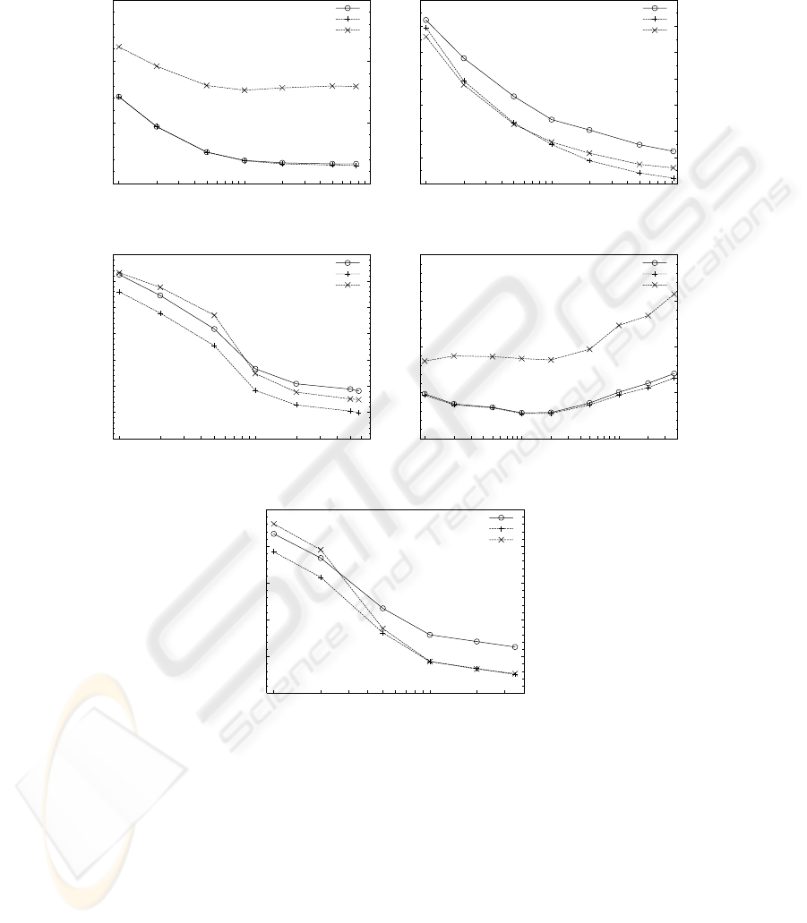
Fig.1. Naive Bayes classification error rate as a function of the vocabulary size for the five
datasets considered. Each plotted point is an error rate averaged over ten 80%-20% train-test
splits. Each panel contains three curves: one corresponds to conventional parameter estimates
(relative frequencies) and the other two refer to maximum entropy (conditional maximum likeli-
hood) training using the GIS algorithm.
63

Table 1. Basic information on the datasets used in the experiments. (Singletons are words that
occur once; Class n-tons refers to words that occur in n classes exactly).
Job 20 Industry 4 7
Category Newsgroups Sector Universities Sectors
Type of documents
job titles & newsgroup web web web
descriptions messages pages pages pages
Number of documents 131643 19974 9629 4199 4 573
Running words 11221K 2549K 1834K 1090K 864K
Average document length 85 128 191 260 189
Vocabulary size 84212 102 752 64551 41763 39375
Singletons (Vocab.%) 34.9 36.0 41.4 43.0 41.6
Classes 65 20 105 4 48
Class 1-tons (Vocab.%) 49.2 61.1 58.7 61.0 58.8
Class 2-tons (Vocab.%) 14.0 12.9 11.6 17.1 11.7
After preprocessing, ten random train-test splits were created from each dataset,
with 20% of the documents held out for testing. Both, conventional and conditional
maximum likelihood training of the naive Bayes model were compared in each split,
using a training vocabulary comprising the top D most informative words in accor-
dance to the information gain criterion [9] (D was varied from 100, 200, 500, 1000,
. . . up to full training vocabulary size). We used Laplace smoothing with ǫ = 10
−5
for conventional training [5], and the GIS algorithm without smoothing for conditional
maximum likelihood training through maximum entropy [10]. The results are shown in
Figure 1. Each plotted point in this Figure is an error rate averaged over its correspond-
ing ten data splits. Note that each plot contains one curve for the conventional training
method and two curves for GIS training: one corresponds to the parameters obtained
after the best iteration and the other to the parameters returned after GIS convergence.
This “best iteration” curve may be interpreted as a (tight) lower bound to the error rate
curve we could obtain by early stopping of the GIS to avoid overfitting.
From the results in Figure 1, we may say that conditional maximum likelihood
training of the naive Bayes model provides similar to or better results than those of
conventional training. In particular, they are significantly better in the Job Category and
4 Universities tasks, where it is also worth noting that maximum entropy does not suffer
from overfitting (the best GIS iteration curve is almost identical to that after GIS conver-
gence). However, in the 20 Newsgroups, Industry Sector and 7 Sectors tasks, the results
are similar. Note that, in these tasks, the error curve for relative frequencies tends to lie
in between the two curves for GIS, which are parallel and separated by a non-negligible
offset (2% in 20 Newsgroups, and 4% in Industry Sector and 7 Sectors). Of course, this
is a clear indication of overfitting that may be alleviated by early stopping of GIS and,
as done for relative frequencies, by parameter smoothing. Another interesting conclu-
sion we may draw from Figure 1 is that, with the sole exception of the 4 Universities
task, the best results are obtained at full vocabulary size. This was previously observed
in [5] for relative frequencies.
Summarising, the best test-set error rates obtained in the experiments are given
in Table 2. These results match previous results usign the same techniques on the five
64

Table 2. Best test-set error rates for the five datasets considered.
Parameter estimation
Smoothed GIS GIS
relative after best after
Dataset frequencies iteration convergence
Job category 32.6 26.3 26.4
20 Newsgroups 13.2 12.4 14.5
Industry-Sector 22.4 19.9 24.1
4 Universities 13.4 7.7 7.8
7 Sectors 17.7 17.6 21.3
datasets considered, though there are some minor differences due to different data pre-
processing, experiment design or parameter smoothing [2,5].
5 Conclusions
We have shown that the naive Bayes and maximum entropy text classifiers are closely
related. More specifically, we have provided a direct, bidirectional link between the
naive Bayes and maximum entropy models for class posteriors. Using this link, max-
imum entropy can be interpreted as a way to train the naive Bayes model with condi-
tional maximum likelihood. We have extended previous empirical tests comparing these
two training criteria. In summary, it may be said that conditional maximum likelihood
training of the naive Bayes model provides similar to or better results than those of
conventional training.
References
1. Lewis, D.: Naive Bayes at Forty: The Independence Assumption in Information Retrieval.
In: Proc. of ECML-98. (1998) 4–15
2. Nigam, K., Lafferty, J., McCallum, A.: Using Maximum Entropy for Text Classification. In:
Proc. of IJCAI-99 Workshop on Machine Learning for Information Filtering. (1999) 61–67
3. McCallum, A., Nigam, K.: A Comparison of Event Models for Naive Bayes Text Classifi-
cation. In: Proc. of AAAI/ICML-98 Workshop on Learning for Text Categorization. (1998)
41–48
4. Juan, A., Ney, H.: Reversing and Smoothing the Multinomial Naive Bayes Text Classifier.
In: Proc. of PRIS-02, Alacant (Spain) (2002) 200–212
5. Vilar, D., Ney, H., Juan, A., Vidal, E.: Effect of Feature Smoothing Methods in Text Classi-
fication Tasks. In: Proc. of PRIS-04, Porto (Portugal) (2004) 108–117
6. Ghani, R.: World Wide Knowledge Base (Web→KB) project. www-2.cs.cmu.edu/
afs/cs.cmu.edu/project/theo-11/www/wwkb (2001)
7. Rennie, J.: Original 20 Newsgroups data set. (www.ai.mit.edu/∼jrennie) (2001)
8. McCallum, A.: Rainbow. (www.cs.umass.edu/∼mccallum/bow/rainbow) (1998)
9. Yang, Y., Pedersen, J.O.: A comparative study on feature selection in text categorization. In:
Proc. of ICML-97. (1997) 412–420
10. Darroch, J., Ratcliff, D.: Generalized Iterative Scaling for Log-linear Models. Annals of
Mathematical Statistics 43 (1972) 1470–1480
65
