
Transductive Support Vector Machines for Risk
Recognition of Sustained Ventricular Tachycardia and
Flicker after Myocardial Infarction
Stanisław Jankowski,
1
Ewa Piątkowska-Janko
2
, Zbigniew Szymański
3
and Artur Oręziak
4
1
Institute of Electronic Systems, Warsaw University of Technology
ul. Nowowiejska 15/19, 00-665 Warsaw, Poland
2
Institute of Radioelectronics, Warsaw University of Technology
ul. Nowowiejska 15/19, 00-665 Warsaw, Poland
3
Institute of Computer Science, Warsaw University of Technology
ul. Nowowiejska 15/19, 00-665 Warsaw, Poland
4
Ist Department of Cardiology, Medical University of Warsaw
ul. Banacha 1 A, 02-097 Warsaw, Poland
Abstract. This paper presents the improved recognition of patients with sus-
tained ventricular tachycardia and flicker after myocardial infarction based on
signal averaged electrocardiography. The novel approach includes: new filter-
ing technique, extended signal description by a set of 9 parameters and the ap-
plication of transductive support vector machine classifier. The dataset consists
of 376 patients selected and commented by cardiologists of the Warsaw Medi-
cal University. The best score 94% of successful recognition on the test set was
obtained for signals filtered by FIR method, described by 9 parameters.
1 Introduction
Ventricular tachycardia is a difficult clinical problem for the physician [4], [5], [9],
[14], [15], [16], [17], [18]. Patients with sustained ventricular tachycardia and ven-
tricular fibrillation have a potential for sudden death. After myocardial infarction the
chance to get sustained ventricular tachycardia or ventricular fibrillation increases,
thus reduction in number of sudden death requires advanced predictive procedures.
The ability to identify properly arrhythmias from signal-averaged ECG (SAECG)[20]
recordings is important for clinical diagnosis and treatment. This paper presents a
novel approach to efficiently and accurately identify normal patients and sustained
ventricular arrhythmias through the SAECG parameters by using the Transductive
Support Vector Machines [6], [15], [21].
Signal-averaged electrocardiography is a technique involving computerized analy-
sis of segments of a standard surface electrocardiogram. [3], [20] Signal-averaging
Jankowski S., Pi ˛atkowska-Janko E., Szyma
´
nski Z. and OrÄ
´
Zziak A. (2007).
Transductive Support Vector Machines for Risk Recognition of Sustained Ventricular Tachycardia and Flicker after Myocardial Infarction.
In Proceedings of the 7th International Workshop on Pattern Recognition in Information Systems, pages 161-170
DOI: 10.5220/0002429501610170
Copyright
c
SciTePress

techniques, which reduce the noise (low-frequency, high-amplitude signals) interfer-
ing with the surface ECG, have been used since the 1970s , and it is used for detect-
ing small electrical impulses, termed ventricular late potentials (VLP), that follow the
QRS segment. Ventricular late potentials in patients with cardiac abnormalities, espe-
cially coronary artery disease or following an acute myocardial infarction, are associ-
ated with an increased risk of ventricular tachyarrhythmias and sudden cardiac death.
The application of support vector machine to the classification of electrocardio-
graphic signals gave excellent results [10], [11]. However, the severe problem deals
with the requirement of labelling the training set examples by cardiologists. Usually
the data set consists of few commented examples and a large set of unlabeled signals.
This fact strongly motivated us to use the transductive approach to medical data rec-
ognition.
2 Transductive Support Vector Machine
Transductive support vector machine (TSVM) is a statistical learning system that
explores the information from the labelled data as well as unlabelled data distribution
in the input space. It is the extension of supervised support vector machine.
The idea of transductive learning was postulated by Vapnik [21] who stated that
transduction – labelling a test set is easier than induction – learning a general rule.
The objective is the classification of unlabelled data by a separating hypersurface
in the Hilbert space between classes with the maximum margin with respect to la-
belled as well as unlabelled data points. The unlabelled points can be assigned to the
class suggested by this solution, named the transductive support vector machine.
Intuitively, we expect that the separating hypersurface is located in the low density
region of unlabelled data points between two classes.
Although the transductive support vector machine defines many new theoretical
and numerical problems (it is NP.-completed problem) the idea is attractive due to
following reasons:
1. The problem is perfectly suited for the applications in medicine [15], bioinformat-
ics [13], text categorization [12] etc., as the data labelling of large data sets is prac-
tically impossible;
2. It is expected that the consideration of unlabelled data distribution can significantly
improve the classifier generalisation with respect to supervised classification, es-
pecially if the number of labelled points is small as compared to the number of
unlabelled points;
3. Semi-supervised classifier has well-defined statistical properties (margin width,
separating border, generalisation), thus it is superior of unsupervised classifiers ob-
tained by some heuristics (e.g. self-organising maps).
There exist some solutions for efficient transductive support vector machines, as
the semi-supervised support vector machine S
3
VM by K. Bennett and Demiriz [2]
that enabled to perform up to several hundreds unlabelled points, SVM-light imple-
mentation of Joachims [12] and large-scale TSVM by Collobert et al. [7] that use
iterative concave-convex procedure (CCCP).
162

The data set consists of l labelled training pairs {(x
l1
, y
l1
),…,(x
ll
, y
ll
)}, x ∈ R
n
,
y ∈ {1, -1} denoted as L set and u unlabelled vectors {x
u1
,…,x
uu
} denoted as U set.
The problem of transductive support vector machine can be performed as an exten-
sion of supervised soft-margin support vector machine by adding 2 constraints to
every point of the working set: One constraint enables to calculate the cost to classifi-
cation error if a given point belongs to the positive class and the second one – the
error cost if a given point belongs to the negative class. The objective function for 2
cases of classification errors is calculated. The minimum cost suggests the labelling
decision of a given unlabelled point. Hence, we deal with the hard combinatorial task.
The primal form of the objective function of linear transductive support vector ma-
chine is as follows:
∑∑
==
++=
l
i
u
j
ji
T
ulunu
CCbyyW
11
****
11
**
1
2
1
),...,,,...,,,,,...,(min
ξξξξξξ
www
(1)
under constraints:
** *
*
*
:( )1
:( )1
:{1,1}
:0
:0
li li i
uj uj j
uj
i
j
iL y b
jU y b
jU y
iL
jU
ξ
ξ
ξ
ξ
∀∈ ⋅ + ≥ −
∀∈ ⋅ − ≥ −
∀∈ ∈− +
∀∈ ≥
∀∈ ≥
wx
wx
where: w, b – parameters of the optimal separating hyperplane,
ξ
,
ξ
*
- slack variables.
The parameters C and C
*
express the trade-off between the margin width and the
number of classification errors on the labelled set data or exclusion of unlabelled data
points. The labels are numbers: +1, −1.
In general, we can introduce a non-linear kernel in order to generalize the trans-
ductive support vector machine. We applied the radial basis function (RBF) kernel
[19]
)||'||exp()',(
2
xxxx −−=
γ
K (2)
The quality of TSVM classifier strongly depends on the proper choice of the pa-
rameters C and C
*
and on the kernel function parameter
γ
.
Our calculations are based on the SVM-light algorithm that operates in the follow-
ing way. The input information consists of labelled data set L and unlabeled set data
U. The parameters set up by the user are: C, C
*
and num+, the predicted cardinal
number of points from positive class of entire set L+U. The algorithm starts from
solving the problem of supervised support vector machine for labelled data set L. The
unlabelled data U are given the labels resulting from the obtained classifier.
The first num+ data points of the largest values of discriminative function:
bKf
l
i
ii
+=
∑
=1
),()( xxx
α
(3)
163
where
α
i
are the Lagrange multipliers of each data point, are assigned to the positive
class and the remaining points to the negative class.
The initially small value of parameter C
*
(10
-5
) is multiplied by 1.5 on each itera-
tion up to the value C set by the user, hence the influence of unlabelled data U on the
position of separating hypersurface grows up. The next loop performs the label
switching caused by some data points and verifies their influence on the objective
function.
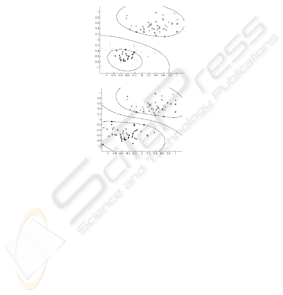
Fig. 1. a) Decision boundary based on small number of labelled examples. b) The decision
boundary is moved to place with low local density: * class +1 examples, + class -1 examples,
{ support vectors, light grey – unlabeled data, black – labelled data.
Therefore the solution is improved by modifying the initial labels of data set points
U in the direction of decreasing objective function. The output of TSVM procedure is
a set of predicted labels of the data set U.
The algorithm is convergent in finite number of label changes due to finite number
of permutations of U points.
The idea of transductive support vector machine is shown in Fig. 1 for a case of
two-dimensional data sets.
3 Signal-averaged ECG Analysis
The Agency for Health Care Policy and Research [1] published a Health Technology
Assessment of SAECG in 1998, concluding that clinical studies of SAECG consis-
164

tently demonstrated a very high negative predictive value (76-100%), variable sensi-
tivity (35-83%) and specificity (47-91%), and poor positive predictive value (8-48%)
when performed on patients with cardiomyopathy or following a myocardial infarc-
tion.
The ability to properly identify arrhythmias from SAECG recordings is important
for clinical diagnosis and treatment, also predictive procedure can reduce the number
of sudden cardiac death.
The method of recording and analysis of SAECG is recommended by the
AHA/ACC/ESC Policy Statement on SAECG Standards, as well as the ACC Expert
Consensus Document on SAECG [5]. After recording x,y,z signals (recommended
Frank leads) the signals are averaged, then filtered using the Bidirectional Butter-
worth Filter. [3] After filtering each lead, x(t), y(t), z(t), the resulting vector magni-
tude (VM) is calculated as (x
2
+ y
2
+ z
2
)
1/2
.
Three time domain parameters were calculated:
1. the total duration of the filtered QRS complex (hfQRS),
2. the root mean square voltage of the last 40 ms of the filtered QRS complex
(RMS40)
3. the duration of the low amplitude (LAS<40 µV) signals at the terminal portion of
the QRS complex.
It was shown that this method has several limitations, as the differences in the al-
gorithms for defining the end and the beginning of QRS, the normal values of men-
tioned parameters and others. [1, 3, 8].
This problem can be solved by using statistical classification method and testing if
we can better extract patients with high risk of ventricular tachyarrhythmia and sud-
den cardiac death. [9] The aim of our study was to improve the method of signal-
averaged ECG for extraction of patients after myocardial infarction with the risk of
sustained ventricular tachycardia by applying different type of filtration and 6 new
parameters. Our study is based on a data set performed at the Chair and Clinic of
Internal Medicine and Cardiology, Warsaw University of Medicine. It consists of 376
patients underwent the signal-averaged ECG recordings. Upon the medical diagnosis,
these patients are divided into 3 groups:
1. patients with sustained ventricular tachycardia (sVT+) after myocardial infarction -
100 patients;
2. patients without sustained ventricular tachycardia (sVT−) after myocardial infarc-
tion - 199 patients;
3. healthy persons – 77 patients.
Only 76 patients from the first group satisfied the common criteria of existence of
late potentials.
4 Time Domain Parameters
The QRS complex of three bipolar leads were combined into the vector magnitude
(Figure 2 and 3). For each of 2 types of filtration (a four-pole IIR Butterworth filter,
FIR filter with Kaiser window) we calculated 9 signal parameters: 3 commonly used
and 6 additional ones, as defined in Table 1.
165
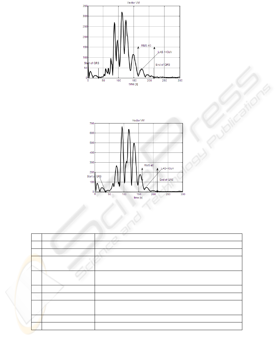
Fig. 2. Example of vector magnitude of filtered QRS complex for patient with sVT+ (four-pole
IIR Butterworth filter).
Fig. 3. Example of vector magnitude of filtered QRS complex for patient with sVT- (four-pole
IIR Butterworth filter).
Table 1. Signal-averaged ECG parameters.
Parameter Definition
1 hfQRS (msec) the total duration of the filtered QRS complex
2 RMS40 (µV) rms voltage of the last 40 ms of the filtered QRS complex
3 LAS<40 µV (ms) the duration of the low amplitude < 40 µV signals at the
terminal portion of the QRS complex
4 LAS<25 µV (ms) the duration of the low amplitude < 25 µV signals at the
terminal portion of the QRS complex
5 RMS QRS (µV) rms voltage of the filtered QRS complex
6 pRMS (µV) rms voltage of the first 40ms of filtered QRS complex
7 pLAS (ms) the duration of the low amplitude < 40 µV signals within
QRS complex
8 RMS t1(µV) rms voltage of the last 10 ms the filtered QRS complex
9 RMS t2 (µV) rms voltage of the last 20 ms the filtered QRS complex
rms – root mean square
166

5 Results
Based on signal-averaged ECG recordings nine data sets described in Table 2 were
created.
Table 2. Description of the data sets.
Data set Number of
parameters
Filtration type
WS3-1,2,t 3 40Hz high-pass and 250Hz low pass four-
pole IIR Butterworth filter
WS9-1,2,t 9 40Hz high-pass and 250Hz low pass four-
pole IIR Butterworth filter
WK9-1,2,t 9 FIR filter with Kaiser window 45-150 Hz
Data sets WS3-t, WS9-t and WK9-t contained 188 cases and were used for testing
of obtained classifiers. Data sets WS3-1, WS9-1 and WK9-1 contained 188 cases and
were used for creation of three supervised SVM models (all data were labelled). Data
sets WS3-2, WS9-2 and WK9-2 contained the same 188 cases as Wxx-1 sets but only
50% of them were labelled. They were used for creation of three TSVM models.
The application runs in Windows system environment. No additional libraries are
required. The input data for the models creation are read from files. The results are
send to standard output of the application. It enables redirection to file for further
analysis or viewing on the screen. The calculations required for the transductive sup-
port vector classifier are much more time consuming than those for the supervised
SVM method due to iterative nature of the TSVM algorithm.
Table 3 contains model properties for the supervised SVM method.
Table 3. Model properties – supervised SVM method.
Data set No. of sup-
port vectors
No. of support
vectors at C
C, gamma Estimation of VC
dimension
WS3-1 25 20 100,
0,5
358,94
WS9-1 26 11 100,
0,5
770,79
WK9-1 24 9 100,
0,5
1010,37
Table 4 contains model properties for the TSVM method. TSVM model contains
fewer support vectors and has higher estimation of VC dimension than equivalent
SVM model.
167

Table 4. Model properties – TSVM method.
Data set No. of sup-
port vectors
No. of support
vectors at C
C, gamma Estimation of VC
dimension
WS3-2 16 12 100,
0,5
423,34
WS9-2 21 8 100,
0,5
664,41
WK9-2 24 6 100,
1
1642,40
The results of classification are listed in Table 5. Each test data set (different from
learning set) was classified by means of regular SVM classifier as well as TSVM
classifier. The results confirm good generalization of obtained models. It is worth to
note that results of SVM and TSVM classification are similar, although only 50% of
data in the second case was labelled. In data set WK-9 the TSVM method achieved
better results.
Table 5. Results of SVM and TSVM classification.
Data set Correct
classifications
[%]
No. of correct
classifications
No. of
misclassifications
SVM TSVM SVM TSVM SVM TSVM
WS3-1,2 92,51 92,51 173 173 15 15
WS9-1,2 92,55 90,43 174 170 14 18
WK9-1,2 93,09 94,15 175 177 13 11
6 Conclusions
This paper reports the study of risk recognition of sustained ventricular tachycardia
and flicker in patients after myocardial infarction based on high-resolution electrocar-
diography. We considered 3 data sets consisting of the signal averaged ECG:
1. filtered by 40Hz high-pass and 250Hz low pass four-pole IIR Butterworth filter
described by three standard parameters,
2. filtered by 40Hz high-pass and 250Hz low pass four-pole IIR Butterworth filter
described by 9 parameters,
3. filtered by FIR filter with Kaiser window 45-150 Hz described by 9 parameters.
We compared the results obtained by the supervised and the transductive SVM
classifier. In all considered cases we obtained very high score of successful recogni-
tion (90-94%). This result is significantly better than 76% obtained by the commonly
used criteria. The best recognition score is obtained for the signal-averaged ECG
recordings filtered by the FIR filter with Kaiser window 45-150 Hz described by 9
parameters. In this case the transductive SVM (TSVM) classifier is superior over the
supervised SVM classifier. All studied support vector classifiers exhibit also excellent
168

statistical properties expressed by small number of support vectors and high value of
estimated VC dimension.
The system is fast enough. The TSVM solution for a data set of several hundreds
points is of order 20-30 seconds, the recognition time is about 0.1 s.
It can be concluded that the transductive support vector machine is an efficient tool
of computer-aided medical data recognition. It enables the improvement of results for
labelled data by exploring much larger set of unlabelled data.
References
1. AHCPR 1998: U.S. Department of Health and Human Services, Public Health Service,
Agency for Healthcare Policy and Research (AHCPR). Signal-averaged electrocardiogra-
phy. Health Technology Assessment No. 11. AHCPR Pub. No. 98-0020. Rockville (MD):
AHCPR; 1998 May
2. Bennett K., A. Demiriz: Semi-supervised support vector machines, Advances in Neural
Information Processing Systems NIPS 12, MIT Press, 1998, 368-374
3. Breithardt G., Cain M., El-Sherif N., et al. Standards for analysis of ventricular late poten-
tials using high resolution or signal-averaged electrocardiography. A statement by a task
force committee of the European Society of Cardiology, the American Heart Association,
and the American College of Cardiology. Circulation 1991. 83 (4): 1481-1488
4. Brembilla-Perrot B. et al.: Value of non-invasive and invasive studies in patients with
bundle branch block, syncope and history of myocardial infarction. Europace (2001) 3,
187–194
5. Cain et al. ACC expert consensus document. Signal Averaged electrocardiography. J.
Amer. Coll. Cardiol 1996; 27:238-49
6. Chapelle O. , B. Schölkopf, A. Zien (eds.): Semi-Supervised Learning, MIT Press, Cam-
bridge, 2006
7. Collobert R., F. Sinz, J. Weston, L. Bottou: Large Scale Transductive SVMs, Journal of
Machine Learning Research 7 (2006), 1687-1712
8. Gomes J.A.: Signal averaged electrocardiography – concepts, methods and applications.
Kluwer Academic Publishers, 1993
9. Heidari H. et all: Analysis of the Sustained Ventricular Arrhythmias from SAECG Using
Artificial Neural Network and Fuzzy Clustering Algorithm; Proc. 20th Annual Interna-
tional Conference of the IEEE Engineering in Medicine and Biology Society, Vol. 20, No
1,1998
10. Jankowski S., J. Tijink, G. Vumbaca, M. Balsi, G. Karpiński: Morphological analysis of
ECG Holter recordings by support vector machines, Medical Data Analysis, Third Interna-
tional Symposium ISMDA 2002, Rome, Italy, October 2002, Lecture Notes in Computer
Science LNCS 2526 (eds. A. Colosimo, A. Giuliani, P. Sirabella) Springer-Verlag, Berlin
Heidelberg New York 2002, pp. 134-143
11. Jankowski S., A. Oręziak, A. Skorupski, H. Kowalski, Z. Szymański, E. Piątkowska-Janko:
Computer-aided Morphological Analysis of Holter ECG Recordings Based on Support
Vector Learning System, Proc. IEEE International Conference Computers in Cardiology
2003, Tessaloniki, pp. 597-600
12. Joachims T.: Transductive Inference for text classification using support vector machines,
Proc. 16
th
International Conference on Machine Learning ICML, San Francisco 1999, 200-
209
169

13. Kasabov N., Shaoning Pang: Transductive Support Vector Machines and Application in
Bioinformatics for Promoter Recognition, Neural Information Processing – Letters and
Reviews, 3 (2004), 31-38
14. Kuchar D.L., Thorburn C.W., Sammel N.L.: Prediction of serious arrhythmic events after
myocardial infarction: signal averaged electrocardiogram, Holter monitoring and radionu-
clide-ventriculography. J. Am. Coll. Cardiol. 1987, 9, 531-538
15. M. Kukar: Transductive reliability estimation for medical diagnosis, Artificial Intelligence
in Medicine 29 (2003), 81-106
16. Oręziak A., M. Niemczyk, E. Piątkowska-Janko, G. Opolski: Detection of Atrial Electrical
Instability in Hypertensive Patients, Computers in Cardiology 30 (2003), 557-560.
17. Oręziak A., Z. Lewandowski, E. Piątkowska-Janko, K. A. Wardyn, G. Opolski: Prediction
Of Serious Ventricular Arrhythmias In Hypertensive Patients With Different Forms Of The
Left Ventricular Geometry; ESC 2005, 3-7.09. 2005
18. Piątkowska-Janko E., A. Oręziak, Z. Lewandowski, , K. A. Wardyn, G. Opolski : Predic-
tion of the Supraventricular Arrhythmias in Hypertensive Patients with Different Forms of
the Left Ventricular , Computers in Cardiology 2006 .
19. Schölkopf B., Smola A.: Learning with Kernels, MIT Press, Cambridge, 2002
20. Simson M B: Signal averaged electrocardiography, in Zipes DP, Jalife J. (Eds): Cardiac
electrophysiology: from cell to bedside. Philadelphia: W.B. Saunders Co., 1990. pp 807-
817
21. V. N. Vapnik: Statistical Learning Theory, Wiley Interscience, New York 1998
170
