
Reliable Biometrical Analysis
in Biodiversity Information Systems
Martin Drauschke
1?
, Volker Steinhage
1
, Artur Pogoda de la Vega
1??
Stephan M
¨
uller
1
, Tiago Maur
´
ıcio Francoy
2? ? ?
and Dieter Wittmann
2
1
Institute of Computer Science, University of Bonn
R
¨
omerstr. 164, 53117 Bonn, Germany
2
Institute of Crop Science and Resource Conservation, University of Bonn
Melbweg 42, 53127 Bonn, Germany
Abstract. The conservation and sustainable utilization of global biodiversity ne-
cessitates the mapping and assessment of the current status and the risk of loss of
biodiversity as well as the continual monitoring of biodiversity. These demands in
turn require the reliable identification and comparison of animal and plant species
or even subspecies. We have developed the Automated Bee Identification System,
which has not only been successfully deployed in several countries, but also sup-
ports taxonomical research as part of the Entomological Data Information Sys-
tem.
Within this framework our paper presents two contributions. Firstly, we explain
how we employ a model-driven extraction of polymorphic features to derive a
rich and reliable set of complementary morphological features. Thereby, we em-
phasize new improvements of the reliable extraction of region-induced and point-
induced features. Secondly, we present how this approach is employed to derive
new important results in biodiversity research.
1 The Role of Identification in Biodiversity Research
Genera and species with ecological or economical use are a very relevant topic in bio-
diversity research. The bees, Apoidea, are of special interest, because about 70% of the
world’s food crops are pollinated by them. The annual value of this pollination service
has been reported to be about 65 billion US-$, cf. [6]. Since there is an alarming ex-
tinction of crop pollinating bees due to diseases, parasites, and pests, as well as due to
human interventions like clearing, pesticides, etc., bees are specially focused by biodi-
versity research.
?
Martin Drauschke is now with the Department of Photogrammetry, Institute of Geodesy and
Geoinformation, University of Bonn, Nussallee 15, 53115 Bonn, Germany
??
Artur Pogoda de la Vega is now with CA Computer Associates GmbH, Emanuel-Leutze-Str.
4, 40547 D
¨
usseldorf, Germany
? ? ?
Tiago Maur
´
ıcio Francoy is now with de Gen
´
etica, Faculdade de Medicina de Ribeir
˜
ao Preto,
USP, Av. Bandeirantes, 3900, 14049-900 Ribeir
˜
ao Preto, SP, Brazil, tfrancoy@rge.fmrp.usp.br
Drauschke M., Steinhage V., Pogoda de la Vega A., Stephan Müller S., Maurício Francoy T. and Wittmann D. (2007).
Reliable Biometrical Analysis in Biodiversity Information Systems.
In Proceedings of the 7th International Workshop on Pattern Recognition in Information Systems, pages 25-36
DOI: 10.5220/0002430300250036
Copyright
c
SciTePress
Due to the worldwide lack of bee exerts (less than 50 experts, so-called bee taxonomists,
worldwide) on the one hand and the urgency of monitoring and protecting endangered
pollinating bee species, the Automated Bee Identification System ABIS has been devel-
oped. After training, ABIS performs a fully automated analysis of images taken from
the forewings of bees. This fully automated analysis is the outanding quality of ABIS
compared with all other approaches, which demand for intensive interactive processing
of each specimen, e.g. [2] or [7]. Compared with these interactive approaches ABIS
has been reported to be at least 50 times more effective since there is no need to adjust
the wings into an exact position of the camera field. The fully automated approach pro-
vides together with the ABIS database an information system for the surveillance and
management of biometrical data of one of the most important pollinating group world-
wide. It has been successfully deployed for monitoring purposes in Germany, Brazil and
the United States, cf. [12]. ABIS is also part of Entomological Data Information Sys-
tem (EDIS), a co-operative research project jointly undertaken by a number of leading
German natural history museums and university institutions in the area of biodiversity
informatics.
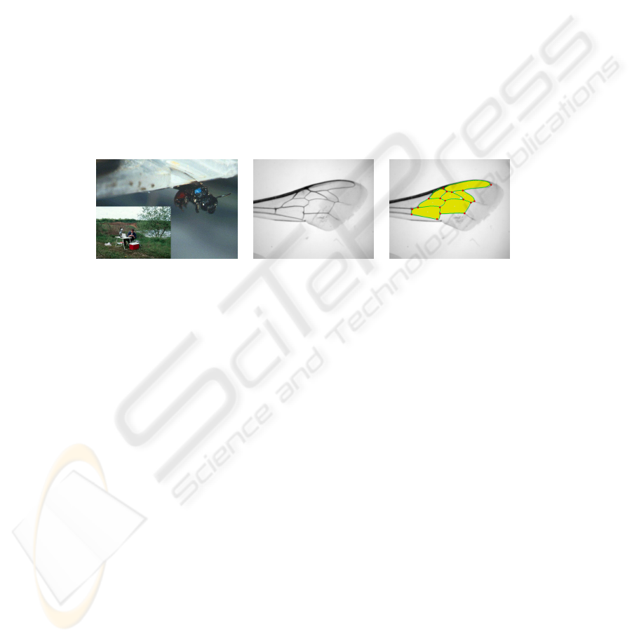
Fig. 1. Left: classification on demand: Bee experts use ABIS during their excursions. Middle:
input image of an Africanized bee. Due to the image aquisition, the scale of all wings is in a
small range. The wing’s position and orientation does not impact the feature extraction. Right:
detected cells and vein net of wing image.
The success of ABIS on identifying bee species leads now to a new challenge: the iden-
tification within the next taxonmical levels, i.e. subspecies and races, which are far more
similar and therefore more difficult to separate. To face this difficult task of subspecies
identification, we improve the extraction algorithms of morphological features, espe-
cially of the region-induced and point-induced features, i.e. cells and vein junctions.
We demonstrate our improved approach within a fascinating taxonomical (oder biodi-
versity) research project on the so-called killer bees. In 1957, swarms of the African
honey bee Apis mellifera scutellata accidentally escaped near Rio Claro, Brazil, and
initiated a series of crosses and backcrosses with the pre-introduced European honey
bee races, cf. [5].
This hybridization process resulted in the Africanized honey bee, which is better adapted
to the tropics and broadly more productive than the European bees. Nevertheless, many
beekeepers abandoned their activities in Brazil at the beginning of the Africanization
process, because these bees presented undesirable traits like a high swarming rate and a
strongly defensive behaviour (which led to their popular, but actually wrong name killer
bees). In the meanwhile, the beekeepers have learnt how to work with these aggressive
bees. Thus, the Africanized honey bee has spread throughout the (sub)-tropic Americas.
26
However, the evolution of the genetic and morphometric profiles of the bees from the
beginning of the Africanization process in Brazil till now is still unknown. The results
of comparing these profiles are not only important in taxonomic terms of biodiversity
research, but may also show important practical implications for pollination manage-
ment and beekeeping.
2 Robust Extraction of Reliable Features
2.1 Basic Steps
The traditional and manual classification approach of bees by taxonomists uses mor-
phological characteristics of their whole body. If a subset of these features enables
an automated, efficient recognition process, we call it a fingerprint. We derive such
a fingerprint from a highly resolved digital image of a bee’s wing as shown in Fig. 1.
The images of the wings typically show under backlight illumination light regions, the
transparent cells, which are surrounded by a dark net: the opaque veins and their junc-
tions. We call the polymorphical features, i. e. the region-induced cells, the line-induced
veins, and the point-induced junctions, primary features. From these primary features,
we compute a set of derived features as listed in Table 1. The set of derived features
forms one part of the fingerprint. On basis of the extracted features, we normalize the
position and orientation of the wing and determine selected grayvalues for the second
part of the fingerprint. The combination of both feature types, the derived features and
the grayvalues, returns the best classification results, cf. [9].
Table 1. List of derived features of the fin-
gerprint.
derived from feature
cells area, circumference,
distance of centers
(absolute and relative values),
eigenvalues and eccentricity
veins length of curvature
junctions distances and angles (along
adjacent cells)
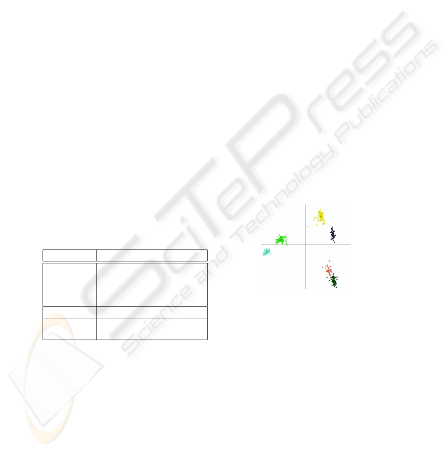
Fig. 2. Demonstration of clusters formed by
fingerprints. Therefore, each feature vector
is projected into a 2D-plane. The samples
of the same subspecies of honey bees are
colored identically.
The expert knowledge is inserted into ABIS within a training step, where genus specific
wing models have to be learnt under supervision of a taxonomist. The wing models con-
tain the expected cell contours including their variance as well as the expected positions
of the vein junctions. Then, ABIS performs a fully automated feature extraction which
consists of the following steps:
1. edge detection using gradient information and
27

2. cell extraction based on grouping of cell border segments until an initial substruc-
ture of cells could be verified by the system, cf. section 2.2,
3. adjusting the trained wing model to the present wing by an affine transformation T ,
4. model-driven cell extraction for difficult cells and
5. precise location of the vein junctions and vein detection, cf. section 2.3,
6. derivation of rotational stable and translation invariant features from extracted cells
and vein net, cf. Tab. 1,
7. statistical analysis of feature vector for bee species classification, cf. [9].
Before starting the classification, we perform a PCA to reduce the dimension of our
feature vector and eliminate redundant information, i.e. if some features are highly cor-
related. Then, the classification can be operated by various discrimination algorithms.
We gained the best results by using the kernel discriminant analyis as proposed by [8].
The integration of the expert knowledge will be done in an offline training step, which
is necessary only once for each classification project. The following tasks must be done
manually within the training step:
1. naming of the extracted cells,
2. identification and naming of the junction positions,
3. fine tuning of classification parameters.
Then, the identification of bee species and subspecies is able to run in a fully automated
way.
In this section, we want to point out the improvements of our feature extraction. Firstly,
star-shaped polygons form an appropriate model of all possible cell shapes. This model
ensures a reliable cell detection, which is based on the grouping of extracted edges.
Secondly, we model the localization of the junctions more precisely. The junctions are
of special importance, because identification by bee experts and by ABIS relays heavily
on the junction positions, i. e. many fingerprint features are derived from them.
2.2 The Use of Star-Shaped Regions for Cell Extraction
Since the border of the cells appear much darker than their inner points, the cell de-
tection starts with an edge detection algorithm, which is based on an approach to line
detection proposed by [11]. This approaches estimates the first and second derivatives
of the image intensity by convolving the image with the derivatives of the Gaussian
smoothing kernel, since this smoothing kernel makes the inherently ill-posed problem
of estimating derivatives of noisy images well posed. In contrast to the line detection
task tackled by Stegers approach, the line-shaped veins of the wing images show lines
with highly variable width - even degenerating into region-shaped areas near the vein
junctions. Therefore, we modify the line detection approach into an edge detection
approach by searching for zero-crossings of the second derivative instead of the first
derivative.
Generally, the detected edge pixels, so-called edgels, do not yield in continuous region
borders. Pseudo veins and disturbances due to hairs and polls on the wings lead to
locally positive false hypotheses of cell borders. Furthermore, mutations and low con-
trasts lead to locally negative false hypotheses of cell borders. Therefore, we developed
28

Fig. 3. Left: all detected edge pixels. Middle: all detected straight edges of a minimum length.
Right: all detected cell hypotheses.
a domain specific grouping strategy. Firstly, we determine all straight edgels of a mini-
mum length, secondly, we classify all other edgels into left and right curved edgels, cf.
Fig. 3.
If some straight edgels are directly connected to right curved edgels at their ends, we
join them to construct cell hypotheses for our cell detection. Our iterative grouping
strategy focuses on the gaps between the current hypotheses on the one hand and the
remaining edgels on the other hand, cf. Fig. 3.
Bee taxonomists can tell us, that the cells in the bee wings are convex or star-shaped.
Hence, we derive the following strategy. Thus, we call a set H of concatenated border
edgels a cell hypothesis, if these concatenated edgels are clockwise ordered around
their center, the mean of all edgels, and if they do not contain a cycle. H denotes the
closed cell hypothesis, where both endings of the cell hypothesis have been connected
by a straight line. The grouping algorithm enlarges each hypothesis H until the closed
border of a region is constructed by the edgels. Two constructive elements of the cell
hypotheses are of interest for the cell detection: the center c(H) and the kernel ker(H)
with
ker(H) =
p ∈ H | ∀x ∈ H : xp ∈ H
, (1)
where xp encodes all points on the straight line between x and p.
The grouping of the border edgels is comparable to a best first search: the algorithm
is looking for the best aggregation with another cell hypothesis for closing the border
of the original cell hypothesis. If the best fitting cell hypothesis does not close the
hypothesis, it must reduce the gap between its endings. The gap size is measured by
the angle α, which is defined by the end point, the center and the start point of the cell
hypothesis.
More precisely, let H
s
be the current cell hypothesis, which has a gap size of α
s
. Then,
in the next iteration step, we determine the new cell hypothesis from H
s
by concatena-
tion with an other appropriate cell hypothesis H
i
, i.e. which has a nearly smooth transi-
tion to H
s
. If there is no such cell hypothesis that closes H
s
to a completely closed cell
border, we append the candidates to resulting hypotheses H
s+1
at either the beginning
or the ending of the start hypothesis, respectively:
H
s+1
= H
i
◦ B ◦ H
s
or H
s+1
= H
s
◦ B ◦ H
i
, (2)
where B encodes the bridging pixels, which form a smooth transition between H
i
and
H
s
. The gap sizes α
s+1
of the resulting hypotheses H
s+1
are determined with the old
29
center c(H
s
) of the start hypothesis, because we want to ensure a decreasing gap size.
We do not recompute the center c
H
s+1
until we have decided for the best fitting cell
hypothesis for aggregation.
When the centers of the cell hypotheses lie in the kernel of the reconstructed cell, this
local inspection works very well. Then, the gap size α
i
decreases monotonously, since
all border points of the region are visible from the center, cf. the corollas on visibility
polygons discussed by [3]. For convex cells, the center of each hypothesis lies in the
kernel of the cell. Since several cells of a bee’s wing are only star-shaped, we need to
shift the center of a cell hypothesis iteratively with each hypothesis update towards the
also iteratively changing kernel of the cell. This task can only be done in a heuristic
way, combining the following two steps:
1. We compute the grayvalue gradient ∇g
c(H)
from the neighborhood of center c(H)
and shift c(H) in the direction of the maximum gradient, until a minimal distance
to the cell border is reached. Especially, this is necessary to move the centers away
from nearly straight hypotheses.
2. The shifted center (from step 1) gets replaced again, now by the mean of the center
itself and both hypothesis’s endings. This step has almost no impact on smaller,
straight hypotheses, but a big one on hypotheses which already form a big part of
a cell. Then, the center of such a hypothesis is pulled towards the opening of the
hypothesis and is now much closer to the center of the extracted cell.
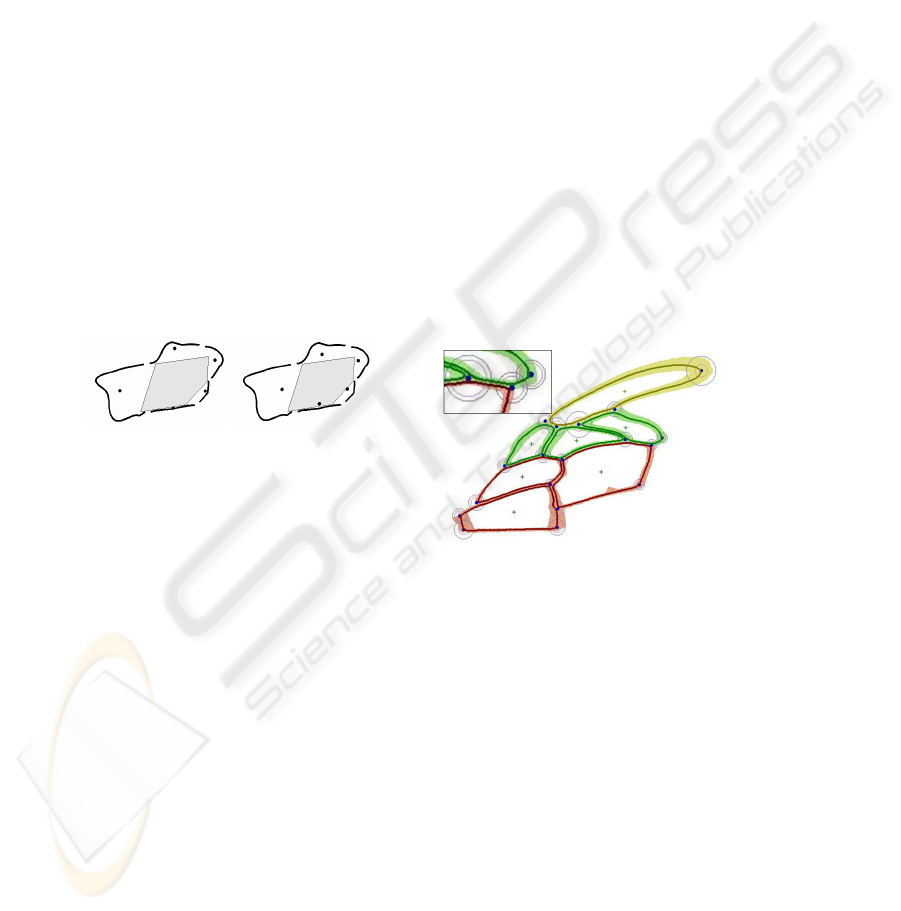
Fig. 4. Five cell hypotheses are shown as black
lines, their centers are visualized by black dots.
Finally, these cell hypotheses should be ar-
ranged together to build the cell. To show the
importance of shifting the centers, we depict
the kernel of the finally reconstructed cell by
the gray filled polygon. The left image shows
the original centers, which are all outside the
kernel - the cell extraction fails in such a case.
The right image shows the centers of the same
cell hypotheses after their transformation - the
cell extraction performs well.
Fig. 5. Wing Model as created in the training
step. The average cell contours are shown by
the darker lines which are surrounded by the
minimum and maximum bounds of the cell
contours. The junctions are set manually into
the wing model.
We show an example in Figure 4, where we need to construct the cell shape from five
cell hypotheses. None of the centers of those hypotheses lies in the kernel of the cell
(left). Our closing procedure originally failed in these cases. Then we extended our
approach and improved the positions of the centers of the cell hypotheses (right). If
the centers were shifted towards the kernel, we were successful with reconstructing the
cell. Nevertheless, in almost all cases, there is a cell hypothesis, whose center lies in the
cell’s kernel after the shifts have been done.
30
We tested our algorithms on about 25,000 cells. Due to the improvements on closing in
the case of non-convex, but star-shaped cells, we are now able to detect all cells of a
bee’s wing in over 99.9% of all tested samples. Fig. 1 shows all detected cells of a wing
image.
The extracted cell borders of all specimens of the training set form the basis for com-
puting the wing model a genus or a group of genera. The wing model describes the
expected cell borders as well as their geometric variances as learnt from the traing set,
cf. Fig. 8. After training the wing model will be employed as a ”road map” for the ex-
traction of cell borders to identify the species or subspecies of speciemens of the trained
genus or group of genera.
2.3 Positioning of the Vein Junctions Using the Wing Template
Classical biometrical approaches show that the appropriate junction positioning is cru-
cial for the successful identification, because a large number of fingerprint features (i.e.
distances, lengths, angles) will be derived from the junction positions, cf. Table 1. Thus,
we have to place the junctions after the complete cell detection.
Therefore, during the training of a wing model, the taxonomist defines exactly the posi-
tions of the junctions into the model, cf. Fig. 5. These positionings will be aligned to the
wing under investigation by the affine transformation T from step 3 of the feature ex-
traction process in section 2. If p is the position of the j-th junction in the wing model,
then p
0
= T p is the estimated position of the junction in the wing.
We estimate the parameters of the affine transformation T from the centers of the cells
in the wing model and the centers of initially extracted cells. These initially extracted
cells are quite robustly to detect without the help of a wing model. They form the basis
for the model-based extraction of the remaining cells together with the generic wing
model. Intutionally, one might say that the inner cells of the wing image are the initially
extracted cells, while the outer cells are the cells, which are more difficult to extract and
therefor we need the wing model. Although, this estimation proved to be locally precise
enough for our purpose, there is a need for readjusting the junction’s coordinates, as
seen in Figure 6. The final position is shown in the right part of Figure 6.
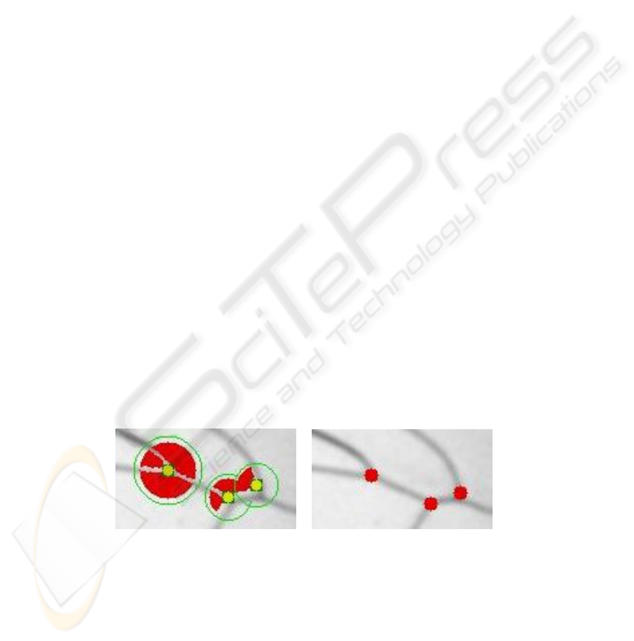
Fig. 6. Left: inprecise localization of junctions by affine transform. Right: final positions of the
junctions after local rearrangements.
The localization of the junctions is improved with the use of explicit, spherical junction
templates, which the bee expert defines also in the wing model. These templates do not
31
only contain the predicted position of a junction, but also its local neighbourhood
E
r
1
(p) := { x | d(x, p) = ||x − p||
2
≤ r
1
} , (3)
and a analogously defined uncertainty area of a junction U
r
2
(p). A junction’s environ-
ment shows the information about the adjacent cells and veins, see Figure 5, Fig. 6, and
Figure 7. Its uncertainty area encodes all valid positions for the junction.
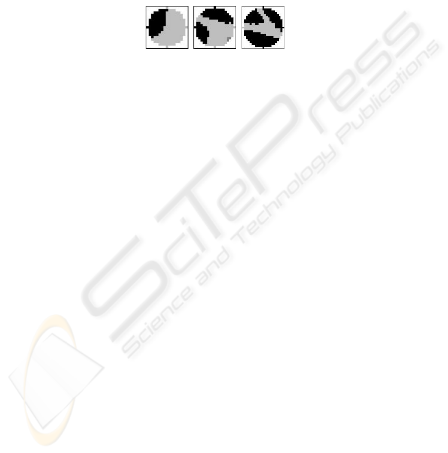
Fig. 7. Visualization of junction templates: E
r
1
contains the adjacent cells in black. The infor-
mation of the veins is derived from the the extruded cells (dilation with a circle, marked in light
gray). Pixels outside of these extruded cells are unknown and marked in dark gray. The examples
show (f.l.t.r.) one, two or three adjacent cells. Thereby, the values of the radii (f.l.t.r. 17, 19 and
23 [pxl]) are chosen by the taxonomic expert and encode the expert knowledge about the relevant
local feature neighbourhood for placing the junctions.
With adjusting of the cells of the wing model to the investigated wing, we also transform
the junction templates. So, we work with affine stable templates for deriving the optimal
positions of the junctions. The two radii r
1
and r
2
, which are chosen by the bee expert,
do not change much by this transformation, so we approximate r
0
1
by r
1
and r
0
2
by r
2
,
respectively.
Considering each pixel in the uncertainty area of a junction z ∈ U
r
2
(p) as a candi-
date for the junction’s position, we perform a template matching by determining the
weighted correlation between the environment E
r
1
(z) and the transformed junction
template. Thus, we shift the junction template such that its center maps to z. Since E
and the template have the same size, we are able to compare them pixel-wise. We define
the following three sets:
– C contains all pixels of E(z), which have been classified as points of cells in the
wing,
– R contains all pixels of E(z), which are marked as points of cells in the shifted
junction template,
– V contains all pixels of E(z), which are marked as points of veins in the shifted
junction template.
Then, we evaluate two functions ρ and ω which are defined on E(z) by
ρ(x) :=
1 , if x ∈ R and x ∈ C
0 , if x /∈ R and x /∈ V
−1 , if x ∈ V and x ∈ C,
(4)
ω(x) :=
1 , if x ∈ V and x /∈ C
0 , else.
(5)
32
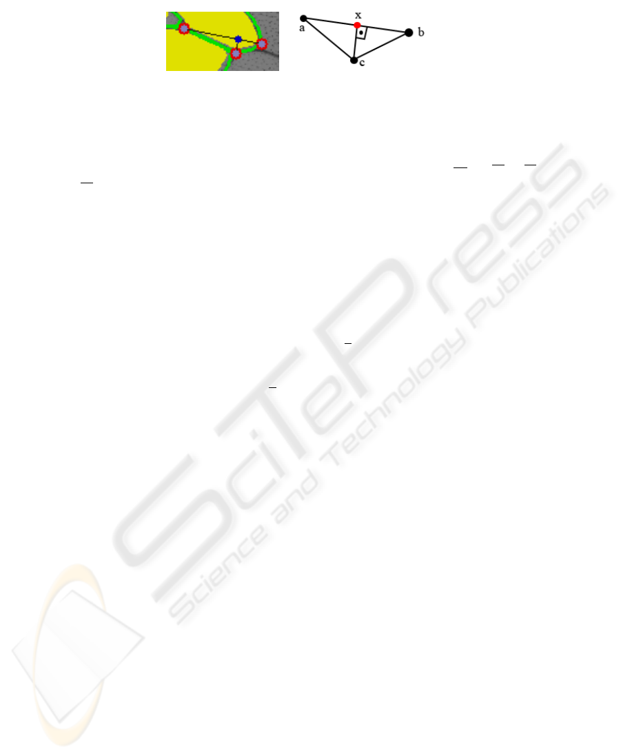
Fig. 8. Selectable derived features: The bee expert has inserted the three junctions a, b and c into
the genus model, e. g. the model for the honey bees. The positions of the three junctions in the
current wing have been placed automatically during the feature extraction. Various fingerprint
features could be derived from these junctions. In a training step for the classification, the bee
expert may select different sets of the derived features. Here, one may choose between two sets
of distances to perpendicular point x for subspecies identification of Apis bees, ax and bx, or ab
and cx. The feature selection may vary between distinct bee genera.
A correspondence between the prediction of the junction template and the classification
of the pixels as cells yields a positive response of ρ(x). Since we do not have any
information on the vein course, we can only consider wrongly classified pixels, where
the template predicts a vein instead of a part of the cell. Then, ρ(x) returns a negative
value for these pixels. The response of ρ(x) is zero, if no information of the pixel is
given by the template.
We obtain the similarity between E and the junction template by
s(z) =
X
x∈E(z)
I(x)
2
ρ(x) + I(x)
2
ω(x), (6)
where I(x) is the intensity value and I(x) is its inverted value. Thus, we combine the
intensity information of the image with ρ- and ω-responses of the template matching.
2.4 Vein Detection
When the detection of the cells succeeded and the placing of the junctions is well done,
the extraction of line-induced veins is relatively simple. As the detected cells and their
shapes have impact on the positional precision of the junctions, they together also in-
fluence the peculiarity of the veins. So, the veins form the complementary space of the
other two feature types. Each vein starts from a junction, runs along the cell borders,
and it ends at a junction. Thus, the thinning approach, which was already proposed in
[9], combined with the idea to connect adjacent junctions around a cell, leads to a highly
reliable detection of the veins.
2.5 Selection of Reliable Fingerprint Features
The classification of bees is based on the fingerprint features, which we derive from the
primary features, i.e. the extracted cells, veins and junctions. Our approach to feature
selection is flexible to cope on different opinions and approaches on relevant feature sets
for morphological identification within the community of taxonomists. Therefore, we
are generally able to derive different fingerprints from the same set of primary morpho-
logical features. Fig. 8 illustrates such a case where we allow the bee expert to derive
different feature sets concerning the honey bees Apis.
33
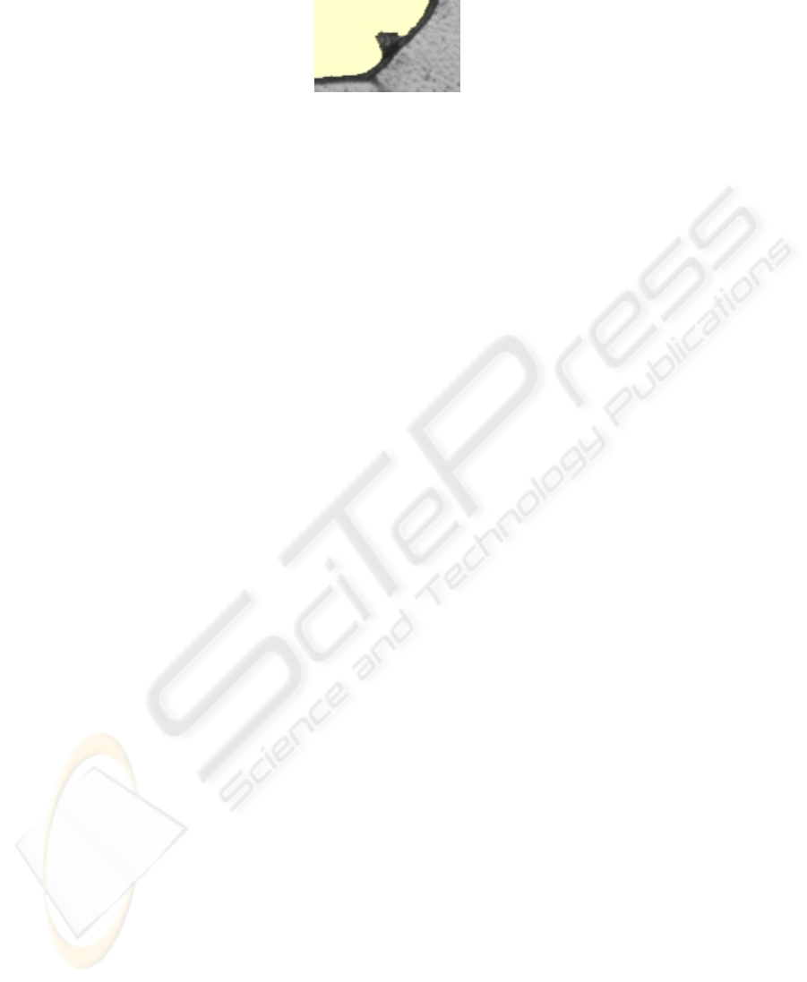
Fig. 9. Data quality inspection: result of the cell extraction of an image with a big pollen inter-
secting a vein. With help of the visualisation, errors like this can be found very easily.
Within the last years, ABIS proved to work successfully using the proposed fingerprint
features as shown in Table 1. Furthermore, the fingerprints are confirmed by our recent
results in subspecies identification.
3 Data Management and Visualization
All the wing images, the primary and derived features, the downsampled images, the
models, identification results and georeferences are maintained with the help of the
ABIS database. As an user-friendly front-end of ABIS and the ABIS-Database, the-
AbisCommander, was developed for the efficient and multimedia-based support of project-
related data management and quality inspection. With the help of AbisCommander, data
can organized easily by drag’n’drop-operations in different projects, thereby providing
the multiple usage of the same data by reference in different projects and roles (i.e.
training, identification), cf. [10].
Visual inspection of input data as well as of all derived data (i.e. features and models)
is important, particularly during the training of wing models. Figure 9 depicts an ex-
tracted deformed cell region caused by a big pollen intersecting one of the veins. Using
this image for training of a wing model, will obviously corrupt the wing model and
therefore decrease classification rates. Such errors can be found easily with help of the
visualization. Generally, AbisCommander can visualize the derived results of each step
in training and identification. Generally, the detection of errors will improve the quality
and reliability of feature extraction and classification.
For the implementation of ABIS and AbisCommander, we paid attention to use open
source software (Java, MySQL, Google Earth) only. This is important, to make ABIS
achievable without great financial investments, which i.e. permits the use in locations
of the third world, where the expert knowledge stored in ABIS is needed mostly.
4 Results, Conclusion, and Outlook
We will now come back to our taxonomical prominent identification project of sub-
species, i.e. the taxonomical research project on the so-called killer bees introduced
in section 1. We use the enhanced ABIS to compare the morphological profile of the
Africanized honey bee population from 1965 with the corresponding profiles of the
most important ancestors populations and the actual one. We work with six groups:
Apis mellifera mellifera, Apis mellifera ligustica, Apis mellifera carnica, Apis mellifera
34
scutellata, Africanized Bees Ribeir
˜
ao Preto (1965), Africanized Bees Ribeir
˜
ao Preto
(2002).
The first three groups represent the most important European ancestor subspecies, while
the fourth group represents the most important African ancestor subspecies. The fifth
and sixth group represent Africanized honey bee populations from 1965 and 2002, re-
spectively. While ABIS was employed successfully for species identification with about
5000 specimens, in this investigation in subspecies level about 100 individuals of each
group were available. After the training ABIS reveals a recognition rate of about 94%
(leave one out test), which is on the one hand “only” 94% due to the very close rela-
tionship of all six groups, but on the other hand sufficient and clearly better than results
of other morphometric approaches.
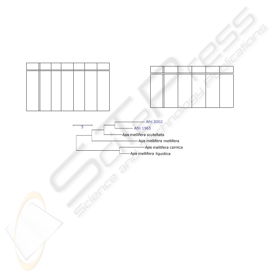
Table 2. Left: confusion matrix of classification with ABIS. Right: Mahalanobis square distances
between the cluster centroids in feature space. We considered the following subspecies of Apis
mellifera: carnica (A.c.), ligustica (A.l.), mellifera (A.m.), scutellata (A.s.), and the Africanized
honey bees from 1965 (A 65) and 2002 (A 02), resp.
A.c. A.l. A.m. A.s. A 65 A 02
A.c. 14.8 0.5 0.0 0.4 0.0 0.0
A.l. 2.5 3.3 0.0 0.0 0.0 0.0
A.m. 0.4 0.0 15.7 0.2 0.0 0.0
A.s. 0.0 0.0 0.2 21.4 0.5 0.0
A 65 0.0 0.0 0.0 0.0 15.8 0.5
A 02 0.0 0.0 0.0 0.2 0.5 23.1
A.c. A.l. A.m. A.s. A 65
A.l. 9.32
A.m. 34.54 29.68
A.s. 27.08 23.65 22.47
A 65 32.98 29.83 21.60 12.40
A 02 37.68 34.04 24.18 15.14 12.43
Fig. 10. Dendrogram showing the Mahalanobis square distances between the two Africanized
honey bee populations of 1965 and 2002 and the ancestor populations.
The tables in Tab. 2 show a more detailed analysis in form of a confusion matrix and
the Mahalanobis square distances between the cluster centroids in feature space, resp.
The very similar and very hardly separable subspecies of Apis m. carnica and Apis m.
ligustica yield the least distance in feature space and the most misclassifications. On the
one hand this missclassification of about 6% will motivate future work on ABIS. On the
other hand the correct results on the other 94% of specimens allow a new taxonomical
interpretation on the basis of the Mahalanobis distances as follows, cf. Tab. 2, and Fig.
10 and [1]:
– The African honey bee A.m. scutellata contributed most to the Africanized popula-
tions.
– A.m. mellifera is the European subspecies that contributed the most to both African-
ized populations. This confirms results from allozymes,
35

– The “mellifera” genes were probably added to the Africanized profile only at the
beginning and spread together with the population.
– The 2002 Africanized population at Ribeir
˜
ao Preto acquired a unique morphometric
profile.
– Since 1965 its distance to the A.m. scutellata and the European ancestors has in-
creased.
The changes in wing venation indicate that the African honey bees continued to dif-
ferentiate from 1965 to 2002 with the effect that the actual populations of the African-
ized bees evolved a unique profile which will keep on changing. The fingerprint of the
Africanized honey bee, which we derived by morphometric analysis of the bee’s wings
using ABIS, shows a significant difference to all the other introduced Apis subspecies
in Brazil. Our results are partially in agreement with results obtained on genetic mark-
ers, e. g. [4] and are initiating further research using genetic markers to confirm our
morphometric results.
References
1. Francoy, T.M., Goncalves, L.S., Wittmann, D.: Changes in the Patterns of Wing Venation
of Africanized Honey Bees over Time. In: VII ENCONTRO SOBRE ABELHAS, 2006,
Ribeir
˜
ao Preto. Anais do VII Encontro sobre Abelhas (2006) 173–177
2. Gauld, I.D., O’Neill M.A., Gaston, K.J.: Driving Miss Daisy: the performance of an auto-
mated insect identification system. In: Austin, A.D., Dowton M. (eds.): Hymenoptera: Evo-
lution, Biodiversity and Biological Control. CSIRO, Canberra (2000) 303–312
3. Goodman, J., O’Rourke, J.: The Handbook of Discrete and Computational Geometry. CRC
Press LLC (1997) 467–479
4. Lobo, J.A., Krieger, H.: Maximum-Likelihood Estimates of Gene Frequences and Racial
Admixture in Apis melifera L. (Africanized Honeybees). Heredity, Vol. 68 (1992) 441–448
5. Perez-Castro, E.E., May-Itz
´
a, W.J., Quezada-Eu
´
an, J.J.G.: Thirty Years after: a Survey on
the Distribution and expansion of Africanized honey bees (Apis mellifera in Peru. J. Apic.
Res., Vol. 41 (2002) 69–73
6. Pimentel, D., Wilson, C., McCullum, C., Huang, R., Dwen, P. , Flack, J., Tran, Q., Salt-
man, T., Cliff, B.: Economics and environmental benefits of biodiversity. Biological Sci-
ences, Vol. 47 11 (1997) 747–757
7. Rohlf, F.J.: tpsDig, digitize landmarks and outlines, version 2.0. Department of Ecology and
Evolution, State University of New York at Stony Brook (2004)
8. Roth, V., Steinhage, V.: Nonlinear Discriminant Analysis Using Kernel Functions. In: Ad-
vances on Neural Information Processing Systems, NIPS ’99, Denver (1999) 568–574
9. Roth, V., Pogoda, A., Steinhage, V., Schr
¨
oder, S.: Integrating Feature-Based and Pixel-Based
Classification for the Automated Identification of Solitary Bees. In: Musterkennung, DAGM
’99, Bonn (1999) 120–129
10. Seim, D., M
¨
uller, S., Drauschke, M., Steinhage, V., and S. Schr
¨
oder: Management and Visu-
alization of Biodiversity Knowledge. In: Proc. 20th International Conference on Informatics
for Environmental Protection, EnviroInfo 2006, Graz, Shaker (2006) 429–432
11. Steger, C.: An Unbiased Detector of Curvilinear Structures. PAMI, Vol. 20 2 (1998) 113–125
12. Steinhage, V., Schr
¨
oder, S., Roth, V., Cremers, A.B., Drescher, W., Wittmann, D.: The
Science of “Fingerprinting” Bees. In: German Research - Magazine of the Deutsche
Forschungsgesellschaft 1 (2006) 19–21
36
