Experiments about the Generalization Ability of
Common Vector based Methods for Face Recognition
?
Marcelo Armengot, Francesc J. Ferri and Wladimiro D
´
ıaz
Dept. d’Inform
`
atica, Universitat de Val
`
encia
Dr Moliner, 50 46100 Burjassot, Spain
Abstract. This work presents some preliminary results about exploring and propos-
ing new extensions of common vector based subspace methods that have been re-
cently proposed to deal with very high dimensional classification problems. Both
the common vector and the discriminant vector approaches are considered. The
different dimensionalities of the subspaces that these methods use as intermedi-
ate step are considered in different situations and their relation to the generaliza-
tion ability of each method is analyzed. Comparative experiments using different
databases for the face recognition problem are performed to support the main
conclusions of the paper.
1 Introduction
There is a number of pattern classification methods that are supposed to deal with very
high dimensional data by means of projecting the original data in appropriate subspaces
fulfilling certain properties. In particular, some of these methods rely on the fact that
dimensionality is (much) larger than the number of available samples in each class.
This is usually known as the small sample size problem[1]. This is the case of the face
recognition problem when faces are processed as vectors of pixels and then each face
can be seen as a point in a very high dimensional space where features are supposed to
correspond to specific parts of faces.
Classical approaches using Principal Component Analysis (PCA) and Linear Dis-
criminant Analysis (LDA) and extensions have been applied to face recognition. One
of the first methods that are worth mentioning is known as the Eigenfaces approach [2]
in which PCA is used to project faces in a lower dimensional space where noise and
small variations are discarded. Using LDA instead of PCA has been also proposed to
keep discriminant information instead. As directly applying LDA is seldom possible in
practice, many different ways of making this feasible gives rise to different approaches
as Fisherfaces [3], the Null Space method [4] or the PCA+NULL method [5].
Methods based on the concept of common vectors have been recently proposed for
classification problems in high dimensional spaces like speech and face recognition [6–
8]. Common vector methods can be thought of as projection methods that make all
samples of a particular class to collapse on a single point (the common vector). In this
subspace, the classification of test samples can be based on their (usually Euclidean)
?
This work has been partially supported by Spanish project DPI2006-15542-C04-04.
Armengot M., J. Ferri F. and Díaz W. (2007).
Experiments about the Generalization Ability of Common Vector based Methods for Face Recognition.
In Proceedings of the 7th International Workshop on Pattern Recognition in Information Systems, pages 129-137
DOI: 10.5220/0002432401290137
Copyright
c
 SciTePress

distance to the common vector in the appropriate subspace. The reason by which this
distance is a good candidate to represent the degree of membership to a particular class
has never been deeply studied.
The goal of this work is to analyze the two main common vector based methods
and compare different options to define classification rules from common vectors and
compare the results with some other subspace-based methods. The paper is organized
as follows. The next section briefly presents the technicalities of the methods involved.
The section 2.2 includes the different options to define the corresponding classification
rules. The experimental comparison is carried out in Section 3 and final conclusion and
further work is given in Section 4.
2 Subspace Methods and Common Vectors
Let suppose we have given m
k
samples in IR
n
(with m
k
≤ n) corresponding to the
k-th class, {x
k
i
}
m
k
i=1
and k = 1, . . . , c.
Let us refer now to a particular class and drop the superscript k. It is possible to
represent each x
i
as the sum
x
i
= x
o
+ ˆx
i
in which the common vector, x
o
, represents the invariant properties common to all
samples of the class and ˆx
i
, called the remaining vector, represents the particular trends
of this particular sample.
The decomposition above corresponds to the projection of x
i
onto two orthogonal
subspaces whose direct sum gives the whole representation space, IR
n
.
These projections can be written in terms of the orthonormal projection operator
P and its orthogonal complement P
⊥
, where P = U U
T
and U = [u
1
, . . . , u
r
] is the
n × r matrix formed with the r eigenvectors corresponding to nonzero eigenvalues of
the k-th class covariance matrix, φ
k
.
In other words, x
o
is the projection of x
i
onto the n − r-dimensional null space of
φ
k
and ˆx
i
is the projection onto the corresponding range space (of dimension r).
Instead of computing x
o
as P
⊥
x
i
, it is possible to use the P = U U
T
that usually
involves much less eigenvectors as
x
o
= x
i
− U U
T
x
i
There is also a more convenient way of obtaining U by using the difference sub-
space of each class and the Gram-Schmidt ortho-normalization procedure instead of
eigenanalysis [7].
The above equation projects data onto a linear subspace, Null(φ
k
), and gives the
same common vector, x
o
for all samples x
i
in the training set. When an unseen k-th
class sample, x is projected onto the same subspace, it is assumed that a vector relatively
close to x
o
will be obtained.
The Common Vector approach (CVA) consists of projecting test samples to the null
spaces of covariance matrices of each class and measure Euclidean distances from these
projections and each one of the common vectors in each class and then assign the class
as
130

arg min
k=1,...,c
(||x − P
k
x − x
k
o
||)
This classifier obviously gives 100% accuracy with the training set but its gener-
alization ability depends on how unseen k -th class samples are scattered in the corre-
sponding null spaces and how other class samples are distributed in these subspaces.
Figure 1 shows four common vectors corresponding to one of the experiments per-
formed in Section 3.
Fig. 1. Common Vectors corresponding to 4 of the classes in the AR dataset used.
2.1 The Discriminant Common Vector Approach
The CVA is similar to the Eigenfaces method because of the fact that the projection
tries to represent the information in each class in the best way. No explicit discriminant
information is taken into account.
If we consider the within-class scatter matrix, S
w
, the between-class scatter matrix,
S
b
and the total scatter matrix, S
t
= S
w
+ S
b
, we can think of maximizing the modified
Fisher criterion [8] in the following way:
1. First project data onto the null space of S
w
and obtain a (discriminant) common
vector corresponding to each class.
2. Apply PCA to the common vectors in the corresponding null subspace to maximize
its scatter.
In this case, a unique projection and corresponding subspace is obtained for all
classes. Also, test samples are projected onto the same subspace and the corresponding
(Euclidean) distances from each common vector are supposed to be representative of
their class. By construction, the final subspace obtained in this case has at most c − 1
dimensions which makes the method more appealing and opens the possibility of easily
visualizing the classification problem in particular cases.
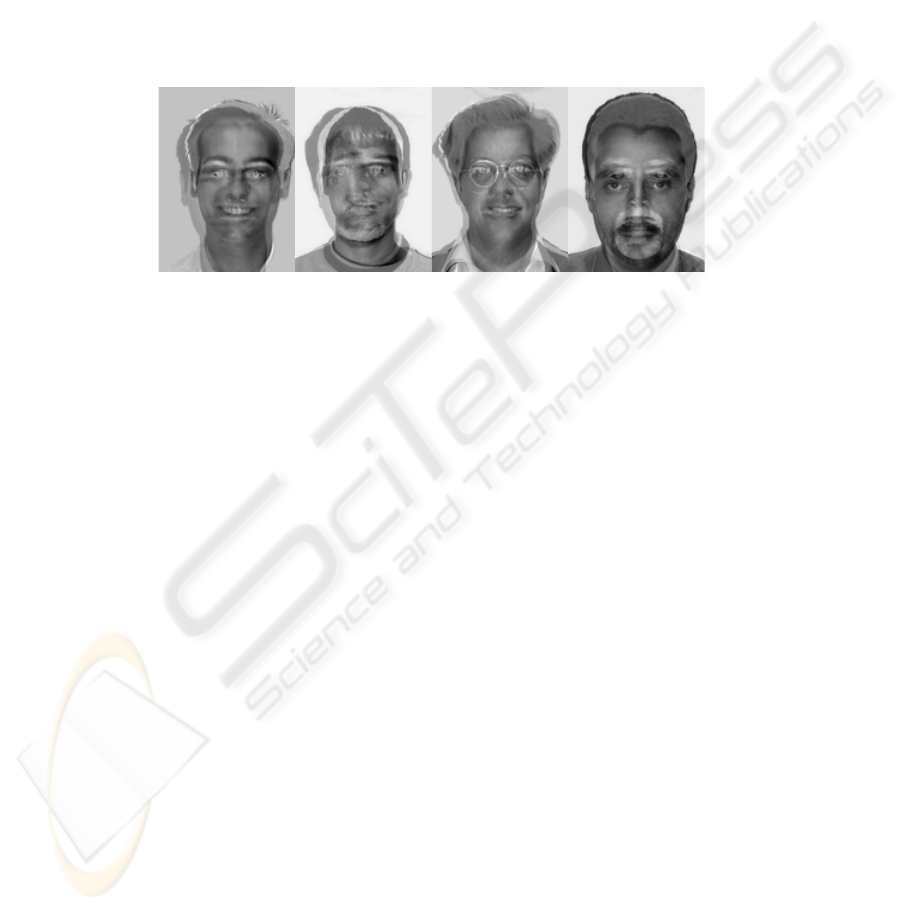
Figure 2 shows four (discriminant) common vectors obtained in the experiments
performed in Section 3.
131

Fig. 2. Discriminant Common Vectors correspondin g to 4 of the classes in the AR dataset used.
2.2 Generalization Ability of Common Vector based Methods
From the formulation of common vector based methods and its properties [7, 8], it is
clear that a 100% recognition rate is obtained on the training set (apart from degen-
erate cases and linear dependences). Once the original dimension has been decreased
(explicitly or implicitly) and all training samples have collapsed to their common vec-
tors, classification is based on the Euclidean distance or variations using angles between
subspaces [7, 9]. In the Euclidean case, this relies on the (strong) assumption that test
samples will be isotropically distributed around its common vector and that all of them
will be closer to it than the projected samples from other classes.
The situation is very different in the two common vector based methods. In the
CVA, there is a different subspace for each class. Moreover, usually the dimension of
these subspaces is quite large (the number of zero eigenvalues or roughly the origi-
nal dimension minus the number of training samples) which can potentially make the
use of Euclidean distance useless. In the DCV there is only one subspace in which all
common vector from all classes lie. Also, this subspace is of relatively low dimension
(the number of classes minus one as all Fisher-based methods). This fact makes pos-
sible to illustrate its behavior for a small 3-class subproblem using data from the AR
database that will be introduced in Section 3. In Figure 3 the (discriminant) common
vector (bold cercles) are shown along with the decision boundaries induced by the min-
imum distance classifier. Several test samples per class are also shown using different
symbols.
It is quite clear from the above explanations and the illustrative example, that the
hypothesis of isotropic distribution is not fulfilled in general (as in most cases when
LDA-based methods are successfully applied). What is worth studying is to which ex-
tent this can be a practical problem and also to start proposing ways to circumvent this
kind of problems.
3 Experimental Results
Three different standard and publicly available databases have been considered in this
work. First, the Olivetti Research Lab (ORL) face database [10], consisting of 10 dif-
ferent views of 40 different individuals is considered. The images have been taken at
different times and with different lighting conditions, facial expressions and details. The
image resolution is 92 × 112 and all images are reasonably aligned.
132

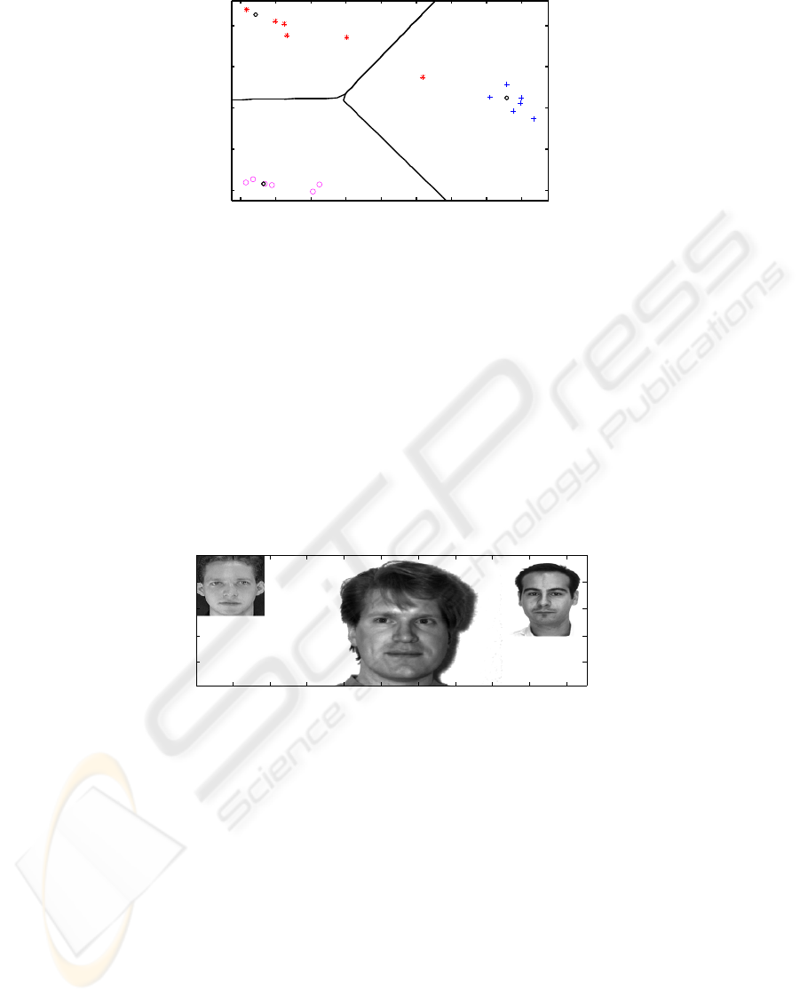
Fig. 3. Test samples and common vectors projected onto the final 2-dimensional subspace corre-
sponding to a 3-class subproblem using the A R database.
Second, the Yale face database [11] contains a total of 165 frontal face images
from 15 different people (11 images per person). Images include also different lighting
conditions, expressions and other details. The resolution is 243 × 320 and images are
approximately aligned. No preprocessing of this database has been made.
Last, the AR face database [12] is considered. This database contains 26 different
views of a number of people from which 20 men and 18 women have been selected
for the experiments. Faces wearing sunglasses or scarfs have been discarded, keeping
only variabilities due to lighting conditions, expressions and time between pictures. The
final size considered is 14 different views of 28 different people. The images have been
down-sampled at 150 × 115 and the margins of the images with no face information
have been trimmed. One example from each one of the databases considered is shown
in Figure 4.
50 100 150 200 250 300 350 400 450 500
50
100
150
200
Fig. 4. Example faces from each of the databases considered in this work. From left to right,
ORL, Yale, and AR.
All databases have been used in the same way, different number of training faces (3,
4, 6, 8 and 9) have been considered and the remaining ones have been used for testing
to obtain holdout estimates of the recognition accuracy of each method. Holdout exper-
iments have been repeated 8, 7, 6, 5 and 5 times (depending on the number of training
faces) and the results have been averaged. All accuracy results shown correspond then
to averaged holdout estimates of the expected accuracy of each method.
Apart from the Common Vector approach (CVA) and the Discriminant Common
Vector method (DCV), other well-known related methods have been considered for
the experiments. In particular, Eigenfaces [2], LDA [11] and Fisherfaces [3] have been
implemented and tested on the same data for comparison purposes. The data has been
133

normalized to have zero mean and unit variance and 95% of the total energy is preserved
when using the Eigenfaces method [11]. The dimension has been reduced to c(m − 1)
using PCA in the Fisherfaces method and standard regularization techniques have been
used to apply the LDA. The nearest neighbor method using the Euclidean distance has
been used in the reduced subspaces to assign the definitive label in all three methods.
2 3 4 5 6 7 8 9 10
0.8
0.85
0.9
0.95
1
1.05
Training Samples
Accuracy
ORL database
Eigenfaces
Fisherfaces
Direct LDA
CVA
DCV
2 3 4 5 6 7 8 9 10
0.65
0.7
0.75
0.8
0.85
0.9
0.95
1
1.05
Training Samples
Accuracy
AR database
Eigenfaces
Fisherfaces
Direct LDA
CVA
DCV
2 3 4 5 6 7 8 9 10
0.4
0.5
0.6
0.7
0.8
0.9
1
1.1
Training Samples
Accuracy
Yale database
Eigenfaces
Fisherfaces
Direct LDA
CVA
DCV
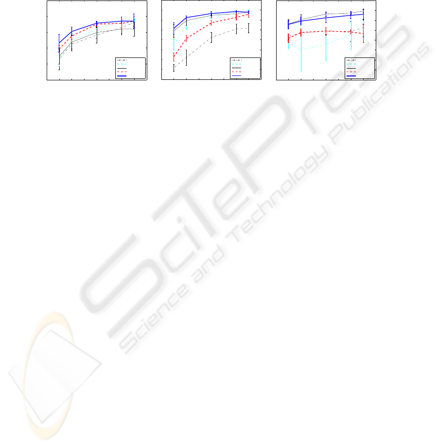
Fig. 5. Accuracies obtained with the three databases for the different methods considered and
different number of training samples.
The results obtained with the five subspace based methods considered on the three
standard databases in the conditions explained above are shown in Figure 5 in one graph
per database. Standard deviations of the averaged holdout estimates of the accuracy are
also displayed.
As can be seen in the figure, all methods give very similar results (no significant
differences) in the case of the (easy) ORL database.
A significant difference can be observed between the two methods based on com-
mon vectors in the other two databases. As it could be expected, the results confirm that
discriminant common vectors consistently gives better results than the plain common
vector approach.
Relatively surprising is the fact that some of the standard methods like (regularized)
LDA and Fisherfaces (in AR database only) give very similar (insignificantly better for
the Yale database) results than the DCV method.
From the computational point of view, the methods considered have very different
behaviors both in training and testing phases. Although the implementations used (us-
ing a very well known matrix based prototyping software system) are by no means op-
timized or programmed in a consistent way that allows strict comparison, approximate
CPU times have been measured for illustrative purposes. These time measurements are
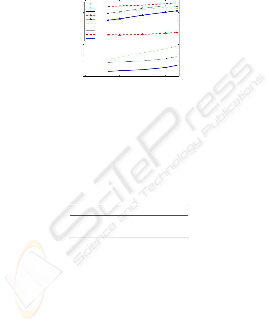
shown in Figure 6. The most outstanding trend in this graph is the high computational
efficiency of the DCV method both in training and testing. The CVA approach shows
the more asymmetric behavior: it is the most efficient in training but by far the slower
in testing.
To study the ability of the different methods to properly generalize, the above ex-
periments have been repeated but adding increasing amounts of noise to the images. In
particular, salt and pepper noise and random (small) rotations and blurring have been
considered only with the AR database. The results obtained are shown in Figure 8 only
134

1 2 3 4 5 6 7 8 9
10
−3
10
−2
10
−1
Yale Database
Training Samples
CPU time
E (tr)
F (tr)
L (tr)
C (tr)
D (tr)
E (ts)
F (ts)
L (ts)
C (ts)
D (ts)
Fig. 6. Approximate CPU times for training (tr) and testing (ts) phases of each of the methods
considered: Eigenfaces (E), Fisherfaces (F), LDA (L), Common Vectors (C) and Discriminant
Common Vectors (D).
for 6 training samples. Note that the results for 0 level noise in both cases are just an-
other random realization of the ones shown in Figure 5. In the case of salt and pepper
noise, the noise level means the probability of having a corrupted pixel. In the second
case, noise level means the amount of degrees (either positive or negative) that a random
rotation of the image can have. Combined with the maximum rotation, a plain average
mask of sizes ranging from 2 to 5. The particular settings used for the results in Figure 8
are shown in Table 1, and an example of an original image from the AR database and
some maximally corrupted images is shown in Figure 7.
Table 1. Settings to generate corrupted images for the experiments to assess generalization ability.
Noise type Noise level
Salt and pepper 0 0.1 0.2 0.3 0.4 0.5
Rot.& blur (degrees) 0 3 6 9 12
Rot.& blur (mask size) 1 2 3 4 5
From this experiment, it is worth noting the ability of the DCV method to deal with
noise. Even when all other methods exhibit a dramatic drop in their accuracy (with a
very very high level of salt and pepper noise), the DCV still gives very similar results.
The differences among methods when a combination of blurring and small random
rotations are are used is not as significant.
135

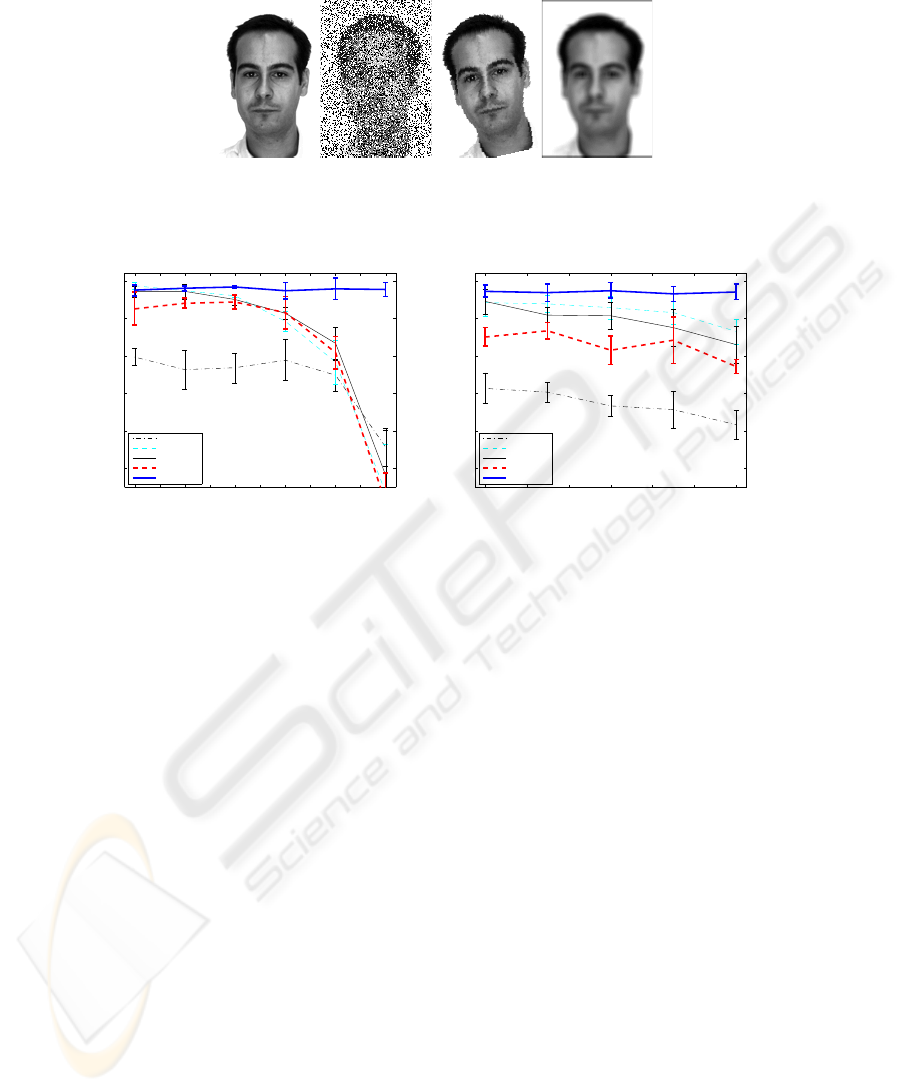
Fig. 7. Example of maximally corrupted images used in the experiment. From left to right: origi-
nal, salt and pepper (0.5), rotated (12
o
) and blurred ( 5 × 5 mask).
0 0.05 0.1 0.15 0.2 0.25 0.3 0.35 0.4 0.45 0.5
0.75
0.8
0.85
0.9
0.95
1
Accuracy
Noise level
AR database (Salt & Pepper)
Eigenfaces
Fisherfaces
LDA
CVA
DCV
0 2 4 6 8 10 12
0.75
0.8
0.85
0.9
0.95
1
Noise level (degrees)
Accuracy
AR database (Rotation & Blur)
Eigenfaces
Fisherfaces
LDA
CVA
DCV
Fig. 8. Results obtained with the AR database with increasing levels of a) salt and pepper and b)
rotation and ll blur noise using all the classification methods considered.
4 Concluding Remarks
In this work, a comparative experimentation of common vector based approaches and
related subspace based methods for face recognition have been considered. The main
features, advantages and drawbacks of these methods have been put forward and their
potential generalization ability has been studied. The experimental setting has been de-
signed on one hand to compare the behavior and computational efficiency of all methods
in several standard databases, and also to open the way to study the generalization abil-
ity of the different approaches. Experiments with increasing levels of different types of
noise have been also conducted to study the way in which the accuracy degrades. The
main preliminary conclusion is that the DCV method is the best option from the differ-
ent point of views. From the particular point of view of generalization, the experiments
performed in this work are clearly insufficient. More experimentation and some particu-
lar proposals to introduce more robust classification rules in the transformed subspaces
are currently on its way.
136

References
1. Fukunaga, K.: Introduction to Statistical Pattern Recognition. Academic Press (1990)
2. Turk, M., Pentland, A.: Eigenfaces for recognition. Journal of Cognitive Neuroscience 3
(1991) 71–86
3. Belhumeur, P.N., Hespanha, J.P., Kriegman, D.J.: Eigenfaces vs. fisherfaces: Recognition
using class specific linear projection. IEEE Trans. Pattern Anal. Mach. Intell. 19 (1997)
711–720
4. Chen, L., Liao, H.M., Ko, M., Lin, J., Yu, G.: A new LDA-based face recognition system
which can solve the small sample size problem. Pattern Recognition 33 (2000) 1713–1726
5. Huang, R., Liu, Q., Lu, H., Ma, S.: Solving the small sample size problem of lda. In: 16th
International Conference on Pattern Recognition. Volume 3. (2002) 29–32
6. Gulmezoglu, M.B., Dzhafarov, V., Keskin, M., Barkana, A.: A novel approach to isolated
word recognition. IEEE Transactions on Speech and Audio Processing 7 (1999) 620–628
7. Gulmezoglu, M.B., Dzhafarov, V., Barkana, A.: The common vector approach and its rela-
tion to principal component analysis. IEEE Transactions on Speech and Audio Processing 9
(2001) 655 – 662
8. Cevikalp, H., Neamtu, M., Wilkes, M., Barkana, A.: Discriminative common vectors for face
recognition. IEEE Transactions on Pattern Analysis and Machine Intelligence 27 (2005) 4 –
13
9. He, Y.H., Zhao, L., Zou, C.R.: Face recognition using common faces method. Pattern
Recognition 39 (2006) 2218–2222
10. Samaria, F., Harter, A.: Parameterisation of a stochastic model for human face identification.
In: 2nd IEEE Workshop on Applications of Computer Vision. (1994)
11. Swets, D., Weng, J.: Using discriminant eigenfeatures for image retrieval. IEEE Trans.
Pattern Anal. Mach. Intell. 18 (1996) 831–836
12. Martinez, A., Benavente, R.: The AR face database. Technical Report 24, Computer Vision
Center, Barcelona (1998)
137