BRAIN COMPUTER INTERFACE
Comparison of Neural Networks Classifiers
Jos´e Luis Mart´ınez P´erez and Antonio Barrientos Cruz
Grupo de Rob´otica y Cibern´etica, Universidad Polit´ecnica de Madrid, C/Jos´e Gutierrez Abascal 2, Madrid, Espa˜na
Keywords:
Electroencephalography, Brain Computer Interface, Spectral Analysis, Biomedical Signal Detection, Pattern
recognition.
Abstract:
Brain Computer Interface is an emerging technology that allows new output paths to communicate the user’s
intentions without use of normal output ways, such as muscles or nerves(Wolpaw, J. R.; et al., 2002).
In order to obtain its objective BCI devices shall make use of classifier which translate the inputs provided by
user’s brain signal to commands for external devices.
The primary uses of this technology will benefit persons with some kind blocking disease as for example:
ALS, brainstem stroke, severe cerebral palsy (Donchin et al., 2000).
This report describes three different classifiers based on three different types of neural networks: Radial Basis
Functions RBF, Probabilistic Neural Networks PNN, and Multi-Layer Perceptrons MLP. The report compares
the results produced by them in order to obtain conclusions to apply to an on-line BCI device, it also describes
the experimental procedure followed in the experiments.
As result of the tests carried out on five healthy volunteers an estimation of the success rate for each type of
classifier, the type and architecture of the classifier, and filtering windows are established.
1 INTRODUCTION
Brain Computer Interface technology(Wolpaw, J.R.;
et al., 2000), BCI, is aimed to communicate human
beings with external computerised devices using the
electroencephalographic signal as primary source of
commands (Birbaumer, N; et al., 2000); in the first
international meeting for BCI technology in 1999 it
was established that BCI “must not depend on the
brain’s normal output pathways of peripheral nerves
and muscles”
In order to control an external device using
thoughts it is necessary to associate some mental pat-
terns to device commands, so an algorithm that de-
tects, acquires, filters and classifies the human elec-
troencephalographic signal is required (Kostov, A.;
Polak, M., 2000) (Pfurtscheller et al., 2000).
This article compares results coming from three
different classifiers based on neural networks: Radial
Basis Function, Probabilistic Neural Networks, and
Multi Layer Perceptron.
In the experiments considered for this article a low
number of electrodes has been used to capture the
endogenous electroencephalographicsubject’s signal.
In order to facilitate the use of this technology it is
important to make it easy to use, the number of elec-
trodes employed in these devices is a global key fea-
ture, as the fewer of electrodes used, the higher the
comfort (Wolpaw, 2007).
Because the main changes in brain activity are as-
sociated to changes in the power amplitude of band
frequencies, spectrograms based on FFT are used to
obtain initial feature vectors (Obermaier et al., 2001)
(Proakis and Manolakis, 1997). Principal Compo-
nent Analysis (PCA) is used to combine these ini-
tial features in order to reduce the dimensionality
of the input space. To minimise the leakage ef-
fect seven different types of preprocess windows has
been considered: rectangular, triangular, Blackman’s,
Hamming’s, Hanning’s, Kaiser’s and Tukey’s (Harris,
1978). The existence of statistical evidence in the fea-
ture population associated to different brain activities
3
Luis Martíinez Pérez J. and Barrientos Cruz A. (2008).
BRAIN COMPUTER INTERFACE - Comparison of Neural Networks Classifiers.
In Proceedings of the First International Conference on Biomedical Electronics and Devices, pages 3-10
DOI: 10.5220/0001047700030010
Copyright
c
 SciTePress

has been previously shown (Pe˜na S´anchez de Rivera,
1986) (Martinez, J.L.; et al., 2006).
The results provided by each classifier are com-
pared using the confusion matrix (Duda et al., 2001).
This article is composed of the following sections:
Section 2 briefly describes the methodology.
Section 3 describes the algorithmics used in the
experiments.
Section 4 and 5 present and analyse the results.
Section 6 is devoted to conclusions.
2 EXPERIMENTAL PROCEDURE
The tests described below were carry out on five male
healthy subjects, one of them has been trained before,
but the other fourwere novice in the use of the system.
In order to facilitate the mental concentration on
the proposed activities, the experiments were carried
on in a room with low level of noise and under con-
trolled environmentalconditions, all electronic equip-
ments external to the experiment around subject were
switched off to avoid electromagnetic artifacts. The
experiments were carry out between 10:00 a.m. and
14:00 p.m. The subjects were sat-down in front of the
acquisition system monitor, at 50 cm from the screen,
their hands were in a visible position, the supervisor
of the experiment controlled the correct development
of it.
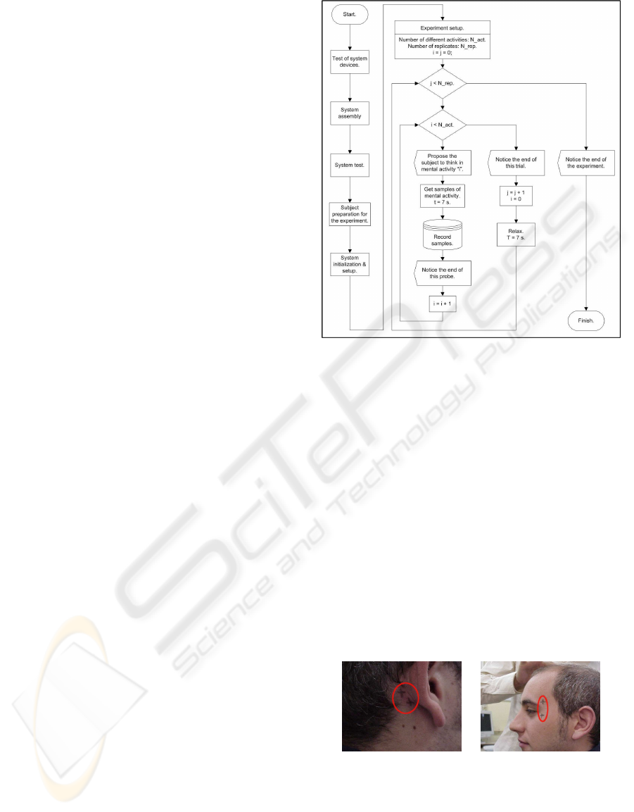
2.1 Methodology
The experimental process is shown on figure 1.
Test of system devices. Checks the correct level of
battery, and the correct state of the electrodes.
System assembly. Device connections: superfi-
cial electrodes (Grass Au-Cu), battery, bio-amplifier
(g.BSamp by g.tec), acquisition signal card (PCI-
MIO-16/E-4 by National Instrument), computer.
System test. Verifies the correct operation of the
whole system. To minimise noise from the electrical
network the Notch filter (50Hz) of the bio-amplifier is
switched on.
Subject preparation for the experiment. Applica-
tion of electrodes on subject’s head. It is verified that
electrode impedance was lower than 4 KOhms.
System initialisation and setup. Verification of
data register. The temporal signal evolution is moni-
tored, in the spectrogram should appear a very low 50
Hz component.
Experiment setup. The supervisor of the experi-
ment sets-up the number of replications, N
rep
= 10,
and the quantity of different mental activities. The
Figure 1: Diagram of the experiment realization.
duration of each trial is t = 7s, the acquisition fre-
quency is f
s
= 384Hz. The system suggests to the
subject to think about the proposed mental activity. A
short relax is allowed at the end of each trial; between
replications the relax time is t = 7s.
2.2 Position of Electrodes
Electrodes were placed in the central zone of the
skull, next to C3 and C4 (Penny, W. D.; et al., 2000),
two pair of electrodes were placed in front of and
behind of Rolandic sulcus, this zone is one with the
highest discriminant power, it takes signal from motor
and sensory areas of the brain (Birbaumer, N; et al.,
2000). Reference electrode was placed on the right
mastoid, two more electrode are placed near to the
corner of the eyes to register blinking.
Figure 2: Electrode placement.
2.3 Description of Cerebral Activities
The supervisor of the experiment asks the subject to
figure out the following mental activities, these ac-
tivities will be the cerebral patterns to differentiate
among them(Neuper, C.; et al., 2001).
BIODEVICES 2008 - International Conference on Biomedical Electronics and Devices
4

Activity A. Mathematical task. Recursive subtraction
of a prime number, i.e. 7, from a big quantity, i.e.
3.000.000.
Activity B. Movement task. This task is subdivided
in:
B-1 Movement imagination. The subject imagines
moving their limbs or hands, but without the materi-
alisation of the movement.
B-2 Movement realization.. The subject is able to
move their hands.
Activity C. Relax. The subject is relaxed.
3 ALGORITHM
This section describes the procedure applied to
recorded signal just before its classification.
Window analysis generator.
Standardization. Windowing.
FFT.
Feature
selection.
registry.
Sample
Neural Networks
Classifier.
Data
base.
Figure 3: Algorithm.
3.1 Window Analysis Generator
In this block the registered signal is chopped in pack-
ages of samples, similar to the bundles of samples ob-
tained from an acquisition card in an on-line BCI ap-
plication. The number of samples in each package is
a compromise between the goodness of the classifica-
tion and the amount of time taken by this classifica-
tion. An algorithm with very good classification and
low number of mistakes will take a very big package,
so the time between classifications will be also very
big, it will do the algorithm useless for a real on-line
BCI system, neither a very fast algorithm with small
packages of samples but with a high number of mis-
takes will be useful.
In this work we have considered packages of 128
samples, the sample frequency is F
s
= 384Hz., and
the classification latency is t = 1/3s.
The duration of each activity is 7s, so there will
be 21 classifications obtained from each register, no
overlap between windows have been considered.
3.2 Standardisation
To compare the signal of different sessions is neces-
sary to standardise the samples, avoiding for exam-
ple that variations in the impedance of the electrodes
changes the classification result.
The standardisation of each analysis window con-
sists in the subtraction of the average value and the
division by the standard deviation.
µ =
Σ
i=N
i=1
x
i
N
; σ
2
=
(x− µ)
2
N
x
′
=
x− µ
σ
3.3 Windowing
In this block different kind of windows are convoluted
with the standardise signal.
The frequency leakage effect occurs when signals
with low frequency components are chopped or con-
voluted with windows with sharp edges, in this cases
in the spectrogram appears high frequency compo-
nents (Harris, F.J., 1978).
The following types of windows have been con-
sidered:
• Rectangular.
• Triangular.
• Blackman’s.
• Hamming’s.
• Hanning’s.
• Kaiser’s.
• Tukey’s.
3.4 FFT
The cerebral activity becomes apparent mainly
through the frequency components of the electro-
encephalographic signal. Different kind of mental ac-
tivities have different frequency components(Harris,
F.J., 1978). For this reason it is necessary to transform
the sampled time domain signal to frequency domain,
so a Fast Fourier Transform is applied to each block
of 2
7
sampled data.
Having in mind that the sample frequency is
384Hz, the frequency resolution is:
∆f =
384Hz
128
= 3Hz.
In this application the useful information is in the
amplitude of the frequencycomponents, so the phases
are discarded, we focus our attention on the spectro-
grams of each of the analysis windows.
Considering the properties of the Fourier Trans-
form and having in mind that the signal in the time
domain only have real components, in the Nyquist
BRAIN COMPUTER INTERFACE - Comparison of Neural Networks Classifiers
5

frequency is produced the reflection effect, so the sig-
nal information is in the first halve of the components
(Harris, F.J., 1978).
3.5 Feature Selection
A vector of features is extracted from each signal
analysis window. This vector is made up as the mean
of the amplitudes of the frequency bands. Because the
frequency of normal human brain is under 40-50Hz,
only frequencies between 6 and 38Hz have been con-
sidered.
Table 1: Feature vector.
FFT index. Frequency. Denomination.
1 0 - 2 Not considered
2 3 - 5 Not considered
3 6 - 8 θ.
4 9 - 11 α
1
.
5 12 - 14 α2.
6 - 7 15 - 20 β
1
.
8 - 10 21 - 29 β
2
.
11 - 13 30 - 38 β
3
.
14 - 64 39 - 192 Not considered
3.6 Classifiers
Three different types of classifiers have been consid-
ered, each one of them based on different types of
neural networks (Ripley, 2000) (Bishop, 1995):
• Multi-Layer Perceptrons (MLP).
• Radial Basis Functions (RBF).
• Probabilistic Neural Networks (PNN).
Each classifier applies the following procedure to
the vector of features extracted previously:
1. Determination of the learning (50%), test (25%)
and validation (25%) sets of data.
2. Attainment of the normalisation matrix for the
learning data set.
3. Application of Principal Component Analysis to
the learning data set in order to reduce the dimen-
sionality of the data input space.
4. Learning of the input data set by the neural net-
work.
5. Application of the neural network to the test data
set, if the error test is bellow the goal error the
learning process is stopped, in other case the net-
work is trained again.
6. Application of the neural network to the valida-
tion data set in order to estimate the performance
error.
7. Application of the neural net to the whole data set
and result registration.
8. Attainment of the confusion matrices for each ex-
periment.
3.6.1 Multi-Layer Perceptron Classifier
The setup parameters used in this classifier are:
• Learning algorithm: Levenberg-Marquardt
(Backpropagation).
• Number of hidden unit neurons: 60.
• Number of output neurons: 3.
• Goal error = 1e
−5
.
• Epochs = 400.
• Max. fail = 5.
• Mem. reduc. = 1.
• Min. grad. = 1e
−10
.
• µ = 1e
−3
.
• µ
dec
= 0.1.
• µ
inc
= 10.
• µ
max
= 1e
−5
.
3.6.2 Radial Basis Function Classifier
The setup parameters used in this classifier are:
• Number of hidden neurons: The learning algo-
rithm used by this type of neural networks deter-
mine the number of neurons in the hidden layer
through an iterative process, it starts with a re-
duced number of hidden neurons and it is in-
creased meanwhile the goal error is not achieved
or a maximum number of neurons is reached.
• Spread constant : 0.25 (Determine the zone of in-
fluence of each neuron).
• Number of output neurons : 3.
3.6.3 Probabilistic Neural Network Classifier
The setup parameters used in this classifier are:
• Number of hidden neurons: The learning algo-
rithm used as much hidden neurons as pairs of
input vector - target vector were in the learning
data set.
• Spread constant : 0.25 (Determine the zone of in-
fluence of each neuron).
• Number of output neurons : 3.
BIODEVICES 2008 - International Conference on Biomedical Electronics and Devices
6

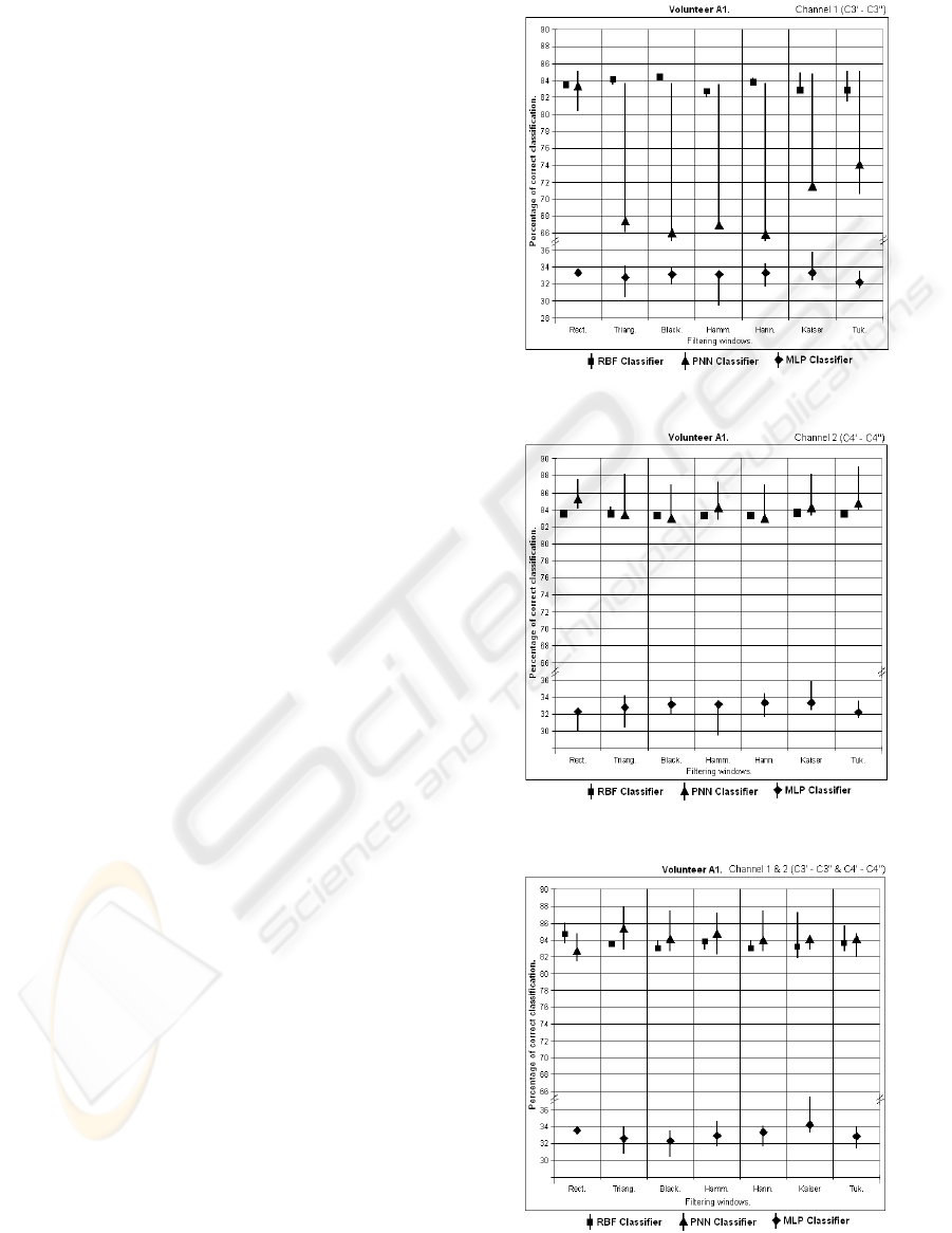
4 RESULTS
The figures in the appendix summarised on vertical
axis the percentage of correct classifications obtained
from the confusion matrices applied to each one of
the three classifiers. It shall be noted that the scale
has been broken in order to appreciate the scattering
results. On the horizontal axis appears the different
types of filtering windows taken into account.
For each filtering window appears a bar with the
results of each classifier: maximum, minimum and
median percentage values.
It is also shown the results obtained when the clas-
sifier use two different types of architectures, one with
only one neuralnetwork that gathersall vectorsof fea-
tures for each electroencephalographic channel, and
other that employs two neural networks, one for each
electroencephalograpic channel.
5 DISCUSSION
From the analysis of the results the following consid-
erations are extracted:
• Classifiers based on Probabilistic Neural Net-
works or Radial Basis Functions perform better
than ones based on Multi Layer Perceptrons.
• Result stability. For all test the procedure was
replicated three times, both PNN and RBF clas-
sifiers produced the same confusion matrices, in-
stead of MLP classifiers which produced different
confusion matrices for each replica.
• Comparison between PNN and RBF classifiers
showed higher maximum percentages of correct
classifications for PNN but also a higher variabil-
ity.
• Classifiers based on only one neural network
that considers at the same time features obtained
from both electroencephalographic channels not
always perform better than classifiers based on
two neural networks, one for each channel.
• Considering the different types of filtering win-
dows, the best results are obtained for Kaiser’s,
rectangular and Tukey’s windows.
6 CONCLUSIONS
This report demonstrates that it is possible to dis-
criminate mental activity from the electroencephalo-
graphic signal, it also compares three different types
of neural networks classifiers applied to an off-line
prototype of BCI device that use FFT in order to esti-
mate the power spectrum of the recorded signal when
volunteers carried out specific mental tasks.
Both classifiers based on Probabilistic Neural Net-
works and Radial Basis Functions produced better
and more stable results than the classifier based on
Multi Layer Perceptrons. It is possible due to the vec-
tor feature distributions associate to each mental ac-
tivity and to the interpolation capability of PNN and
RBF, this capability is higher in PNN and RBF than
in MLP neural networks.
It is hoped that On-line BCI devices based on clas-
sifiers that make use of neural networks like RBF or
PNN will perform better than other based on MLP or
equivalents.
In order to improve the success rate of classifica-
tions the use of filtering windows has been proved to
be a good technique. In the same manner a classi-
fier with a multiple network architecture followed by
a block that weighs the network outputs could pro-
duce better results than classifiers based on only one
neural network.
REFERENCES
Birbaumer, N; et al. (2000). The thought translation device
(TTD) for completely paralyzed patients. IEEE Trans-
actions on Rehabilitation Engineering., 8(2):190–
193.
Bishop, C. (1995). Neural Networks for Pattern Recogni-
tion Analysis. Oxford University Press, London, 1st
edition.
Donchin, E., Spencer, K. M., and Wijesinghe, R. (2000).
The mental prosthesis: assessing the speed of a
p300-based brain-computer interface. Rehabilita-
tion Engineering, IEEE Transactions on [see also
IEEE Trans.on Neural Systems and Rehabilitation],
8(2):174–179.
Duda, R. O., Hart, P. E., and Strok, D. G. (2001). Pat-
tern classification. John Wiley & sons, New York etc.
Richard O. Duda, Peter E. Hart, David G. Strok.
Harris, F. J. (1978). On the use of windows for harmonic
analysis with the discrete fourier transform.
Harris, F.J. (1978). On the Use of Windows for Harmonic
Analysis with the Discrete Fourier Transform. Pro-
ceedings of the IEEE, 66(1):51–83.
Kostov, A.; Polak, M. (2000). Parallel man-machine
training in development of EEG-based cursor con-
trol. IEEE Transactions on Rehabilitation Engineer-
ing., 8(2):203–205.
Martinez, J.L.; et al. (2006). The windowing Effect in
Cerebral Pattern Classification. An Application to
BCI Technology. IASTED Biomedical Engineering
BioMED 2006, pages 1186–1191.
BRAIN COMPUTER INTERFACE - Comparison of Neural Networks Classifiers
7

Neuper, C.; et al. (2001). Motor Imagery and Direct Brain-
Computer Communication. Proceedings of the IEEE,
89(7):1123–1134.
Obermaier, B., Neuper, C., Guger, C., and Pfurtscheller,
G. (2001). Information transfer rate in a five-
classes brain-computer interface. IEEE Transactions
on Neural Systems and Rehabilitation Engineering.,
9(3):283–288. Importante.
Pe˜na S´anchez de Rivera, D. (1986). Estad´ıstica : modelos
y m´etodos, volume 109-110. Alianza, Madrid. Daniel
Pea Sanchez de Rivera; 2 v. 23 cm; 1. Fundamentos –
2. Modelos lineales y series temporales.
Penny, W. D.; et al. (2000). EEG-based communication: A
pattern recognition approach. IEEE Transactions on
Rehabilitation Engineering., 8(2):214–215.
Pfurtscheller et al. (2000). Current trends in Graz brain-
computer interface (BCI) research. IEEE Transactions
on Rehabilitation Engineering., 8(2):216–219.
Proakis, J. G. and Manolakis, D. G. (1997). Tratamiento
digital de seales : [principios, algoritmos y aplica-
ciones]. Prentice-Hall, Madrid.
Ripley, B. (2000). Pattern Recognition and Neural Net-
works. Cambridge University Press, London, 2nd edi-
tion.
Wolpaw, J. R. (2007). Brain-computer interfaces as new
brain output pathways. The Journal of Physiology.
Wolpaw, J. R.; et al. (2002). Brain-Computer interface for
communication and control. Clinical Neurophysiol-
ogy, 113:767–791.
Wolpaw, J.R.; et al. (2000). Brain-Computer Interface Tech-
nology: A Review of the First International Meet-
ing. IEEE Transactions on Rehabilitation Engineer-
ing., 8(2):164–171.
APPENDIX
Figure 4: Channel 1. Correct classification.
Figure 5: Channel 2. Correct classification.
Figure 6: Channel 1 and 2. Correct classification.
BIODEVICES 2008 - International Conference on Biomedical Electronics and Devices
8

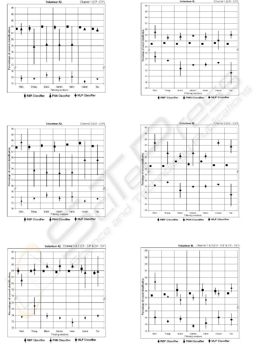
Figure 7: Channel 1. Correct classification.
Figure 8: Channel 2. Correct classification.
Figure 9: Channel 1 and 2. Correct classification.
Figure 10: Channel 1. Correct classification.
Figure 11: Channel 2. Correct classification.
Figure 12: Channel 1 and 2. Correct classification.
BRAIN COMPUTER INTERFACE - Comparison of Neural Networks Classifiers
9

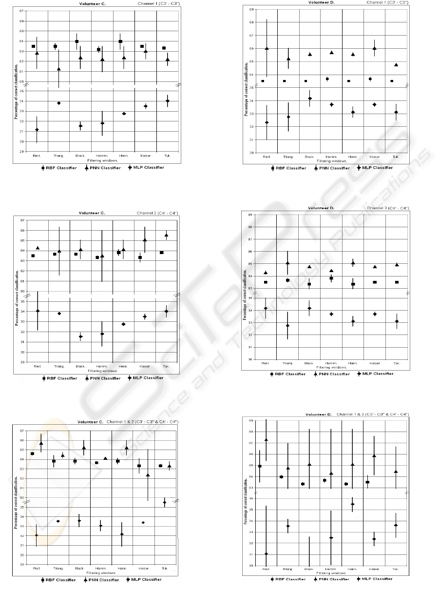
Figure 13: Channel 1. Correct classification.
Figure 14: Channel 2. Correct classification.
Figure 15: Channel 1 and 2. Correct classification.
Figure 16: Channel 1. Correct classification.
Figure 17: Channel 2. Correct classification.
Figure 18: Channel 1 and 2. Correct classification.
BIODEVICES 2008 - International Conference on Biomedical Electronics and Devices
10